Deep learning and unsupervised feature learning have shown great promise in many practical applications. State-of-the-art performance has been reported in several domains, ranging from speech recognition and image recognition to text processing and beyond.
It’s also been observed that increasing the scale of deep learning—with respect to numbers of training examples, model parameters, or both—can drastically improve accuracy. These results have led to a surge of interest in scaling up the training and inference algorithms used for these models and in improving optimization techniques for both.
The use of GPUs is a significant advance in recent years that makes the training of modestly-sized deep networks practical. A known limitation of the GPU approach is that the training speed-up is small when the model doesn’t fit in a GPU’s memory (typically less than 6 gigabytes).
To use a GPU effectively, researchers often reduce the size of the dataset or parameters so that CPU-to-GPU transfers are not a significant bottleneck. While data and parameter reduction work well for small problems (e.g. acoustic modeling for speech recognition), they are less attractive for problems with a large number of examples and dimensions (e.g., high-resolution images).
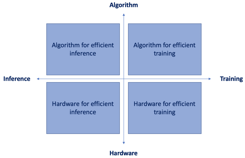
In the previous post, we talked about 5 different algorithms for efficient deep learning inference. In this article, we’ll discuss the upper right part of the quadrant on the left. What are the best research techniques to train deep neural networks more efficiently?
1 — Parallelization Training
Let’s start with parallelization. As the figure below shows, the number of transistors keeps increasing over the years. But single-threaded performance and frequency are plateauing in recent years. Interestingly, the number of cores is increasing.
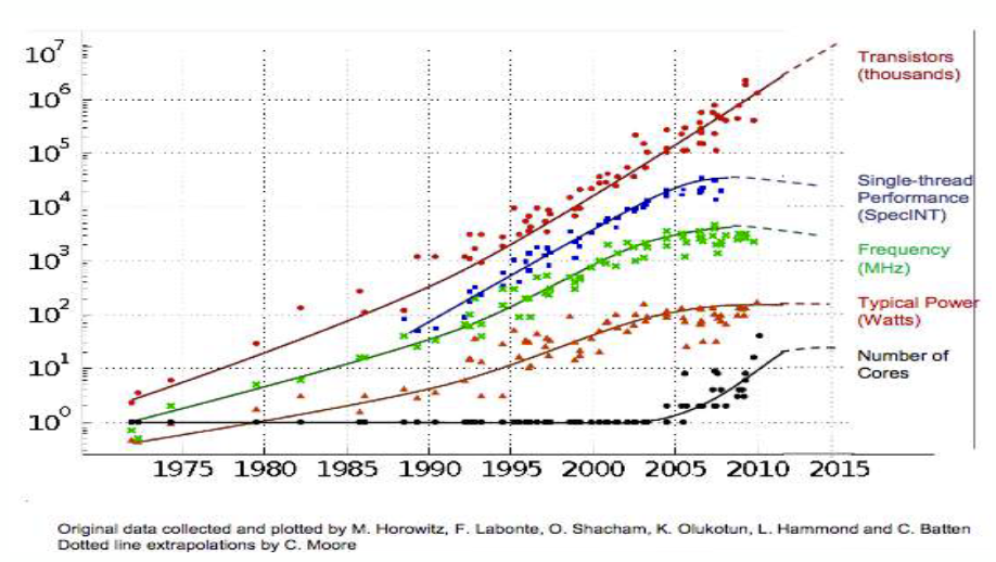
So what we really need to know is how to parallelize the problem to take advantage of parallel processing. There are a lot of opportunities to do that in deep neural networks.
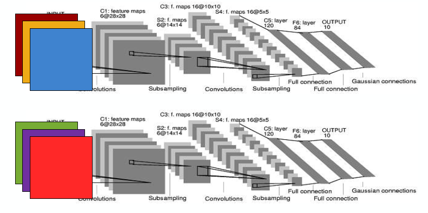
For example, we can do data parallelism: feeding 2 images into the same model and running them at the same time. This does not affect latency for any single input. It doesn’t make it shorter, but it makes the batch size larger. It also requires coordinated weight updates during training.
For example, in Jeff Dean’s paper “Large Scale Distributed Deep Networks,” there’s a parameter server (as a master) and a couple of model workers (as slaves) running their own pieces of training data and updating the gradient to the master.
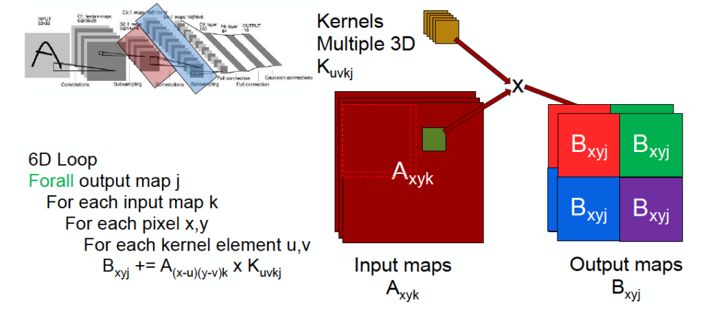
Another idea is model parallelism — splitting up the model and distributing each part to different processors or different threads. For example, imagine we want to run convolution in the image below by doing a 6-dimension “for” loop. What we can do is cut the input image by 2×2 blocks, so that each thread/processor handles 1/4 of the image. Also, we can parallelize the convolutional layers by the output or input feature map regions, and the fully-connected layers by the output activation.
2 — Mixed Precision Training
Larger models usually require more compute and memory resources to train. These requirements can be lowered by using reduced precision representation and arithmetic.
Performance (speed) of any program, including neural network training and inference, is limited by one of three factors: arithmetic bandwidth, memory bandwidth, or latency. Reduced precision addresses two of these limiters. Memory bandwidth pressure is lowered by using fewer bits to store the same number of values. Arithmetic time can also be lowered on processors that offer higher throughput for reduced precision math. For example, half-precision math throughput in recent GPUs is 2× to 8× higher than for single-precision. In addition to speed improvements, reduced precision formats also reduce the amount of memory required for training.
Modern deep learning training systems use a single-precision (FP32) format. In their paper “Mixed Precision Training,” researchers from NVIDIA and Baidu addressed training with reduced precision while maintaining model accuracy.
Specifically, they trained various neural networks using the IEEE half-precision format (FP16). Since FP16 format has a narrower dynamic range than FP32, they introduced three techniques to prevent model accuracy loss: maintaining a master copy of weights in FP32, loss-scaling that minimizes gradient values becoming zeros, and FP16 arithmetic with accumulation in FP32.
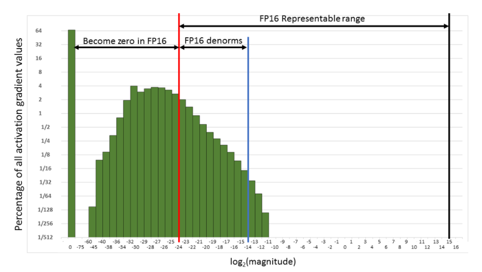
Using these techniques, they demonstrated that a wide variety of network architectures and applications can be trained to match the accuracy of FP32 training. Experimental results include convolutional and recurrent network architectures, trained for classification, regression, and generative tasks.
Applications include image classification, image generation, object detection, language modeling, machine translation, and speech recognition. The proposed methodology requires no changes to models or training hyperparameters.
3 — Model Distillation
Model distillation refers to the idea of model compression by teaching a smaller network exactly what to do, step-by-step, using a bigger, already-trained network. The ‘soft labels’ refer to the output feature maps by the bigger network after every convolution layer. The smaller network is then trained to learn the exact behavior of the bigger network by trying to replicate its outputs at every level (not just the final loss).
The method was first proposed by Bucila et al., 2006 and generalized by Hinton et al., 2015. In distillation, knowledge is transferred from the teacher model to the student by minimizing a loss function in which the target is the distribution of class probabilities predicted by the teacher model. That is — the output of a softmax function on the teacher model’s logits.
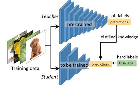
So how do teacher-student networks exactly work?
- The highly-complex teacher network is first trained separately using the complete dataset. This step requires high computational performance and thus can only be done offline (on high-performing GPUs).
- While designing a student network, correspondence needs to be established between intermediate outputs of the student network and the teacher network. This correspondence can involve directly passing the output of a layer in the teacher network to the student network, or performing some data augmentation before passing it to the student network.
- Next, the data are forward-passed through the teacher network to get all intermediate outputs, and then data augmentation (if any) is applied to the same.
- Finally, the outputs from the teacher network are back-propagated through the student network so that the student network can learn to replicate the behavior of the teacher network.
4 — Dense-Sparse-Dense Training
The research paper “Dense-Sparse-Dense Training for Deep Neural Networks” was published back in 2017 by researchers from Stanford, NVIDIA, Baidu, and Facebook. Applying Dense-Sparse-Dense (DSD) takes 3 sequential steps:
- Dense: Normal neural net training…business as usual. It’s notable that even though DSD acts as a regularizer, the usual regularization methods such as dropout and weight regularization can be applied as well. The authors don’t mention batch normalization, but it would work as well.
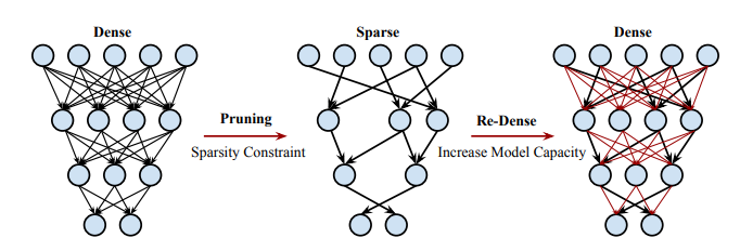
- Sparse: We regularize the network by removing connections with small weights. From each layer in the network, a percentage of the layer’s weights that are closest to 0 in absolute value is selected to be pruned. This means that they are set to 0 at each training iteration. It’s worth noting that the pruned weights are selected only once, not at each SGD iteration. Eventually, the network recovers the pruned weights’ knowledge and condenses it in the remaining ones. We train this sparse net until convergence.
- Dense: First, we re-enable the pruned weights from the previous step. The net is again trained normally until convergence. This step increases the capacity of the model. It can use the recovered capacity to store new knowledge. The authors note that the learning rate should be 1/10th of the original. Since the model is already performing well, the lower learning rate helps preserve the knowledge gained in the previous step.
Removing pruning in the dense step allows the training to escape saddle points to eventually reach a better minimum. This lower minimum corresponds to improved training and validation metrics.
Saddle points are areas in the multidimensional space of the model that might not be a good solution but are hard to escape from. The authors hypothesize that the lower minimum is achieved because the sparsity in the network moves the optimization problem to a lower-dimensional space. This space is more robust to noise in the training data.
The authors tested DSD on image classification (CNN), caption generation (RNN), and speech recognition (LSTM). The proposed method improved accuracy across all three tasks. It’s quite remarkable that DSD works across domains.
- DSD improved all CNN models tested — ResNet50, VGG, and GoogLeNet. The improvement in absolute top-1 accuracy was respectively 1.12%, 4.31%, and 1.12%. This corresponds to a relative improvement of 4.66%, 13.7%, and 3.6%. These results are remarkable for such finely-tuned models!
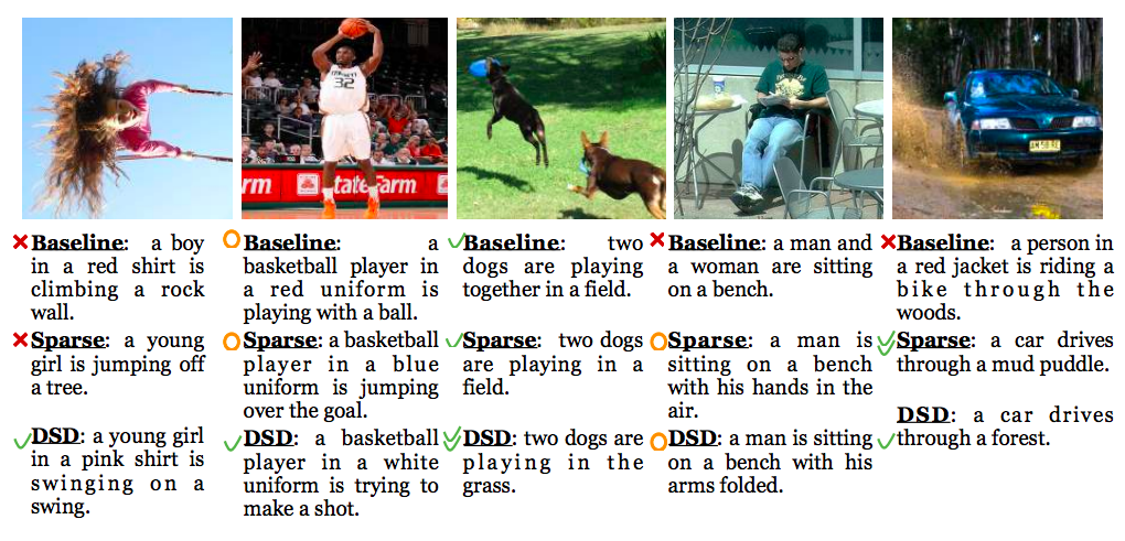
- DSD was applied to NeuralTalk, an amazing model that generates a description from an image. To verify that the Dense-Sparse-Dense method works on an LSTM, the CNN part of Neural Talk is frozen. Only the LSTM layers are trained. Very high (80% deducted by the validation set) pruning was applied at the Sparse step. Still, this gives the Neural Talk BLEU score an average relative improvement of 6.7%. It’s fascinating that such a minor adjustment produces this much improvement.
- Applying DSD to speech recognition (Deep Speech 1) achieves an average relative improvement of Word Error Rate of 3.95%. On a similar but more advanced Deep Speech 2 model Dense-Sparse-Dense is applied iteratively two times. On the first iteration, pruning 50% of the weights, then 25% of the weights are pruned. After these two DSD iterations, the average relative improvement is 6.5%.
Conclusion
I hope that I’ve managed to explain these research techniques for efficient training of deep neural networks in a transparent way. Work on this post allowed me to grasp how novel and clever these techniques are. A solid understanding of these approaches will allow you to incorporate them into your model training procedure when needed.

Comments 0 Responses