Complex models such as deep neural networks are prone to overfitting because of their flexibility in memorizing the idiosyncratic patterns in the training set, instead of generalizing to unseen data.
Any modification we make to a learning algorithm that’s intended to reduce its generalization error but not its training error is called regularization. Keeping the model simple enough by using regularization techniques allows the network to generalize well on data points it hasn’t seen before.
In this article, we’ll discuss the concept of overfitting in deep neural networks and how regularization helps to address the problem of overfitting. We’ll then look at a few different regularizations methods.
The article will be structured as follows:
Overview of regularization
- Why do we need regularization
- Analyzing simple vs complex Model
- Bias-Variance trade-off
- Overfitting in deep neural networks
Regularization methods
- L2 regularization
- Dataset augmentation
- Early stopping
Why do we need regularization?
Before we go into the actual discussion of regularization, we’ll start by learning the concept of bias-variance trade-off.
Let’s assume that we have taken 1D toy data with input (x) & output (y) and there exists a true relationship between input & output y = f(x). For the sake of explanation, assume we know the true relationship between input & output f(x) = sin(x).
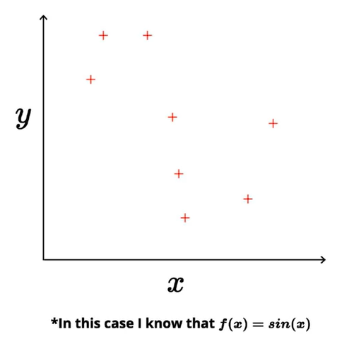
In machine learning/deep learning the goal is to approximate the relationship between input and output. In the case of our toy dataset, we’ll approximate the relationship using two different models — a simple model and a complex model.
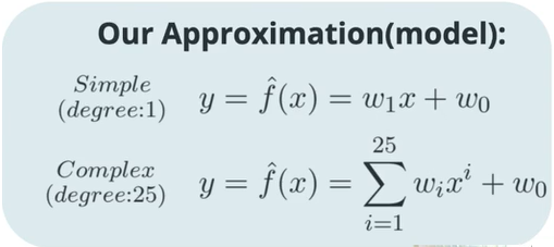
The simple model represents the straight line of the form y = mx + c with only two parameters. The complex model is the 25th-degree polynomial with 26 parameters.
By using these two approximations, we can calculate the predicted value of ‘y’, and then by using the gradient descent algorithm, we can learn the parameters that are best suited for the given data, i.e… the squared error loss for training data would be at its minimum.
Once we know the optimal values of the parameters from gradient descent, we can plug these into our equations to get the best fit curve.
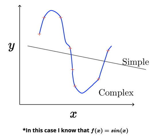
The simple model learned to draw a straight line roughly through the center of the training data so that the average distance between the line and points that lie on above and below the line is at its minimum.
Looking at the complex model, it is able to learn the complex polynomial equation such that it exactly passes through all the training data points. As the complexity of the model increases, the training error reduces to zero, and the complex model tries to memorize the patterns and the noise from the training data.
Analyzing Simple vs Complex Models
Let’s assume that the training data actually consists of 100 points. Say that we sample 25 points (these points are drawn from a sinusoidal function — true relationship) randomly from the training data and train a simple and complex model. Repeat the experiment ‘k’ times to train.
We wouldn’t get the same curve because each time the model sees a different sample of the training data, and the parameters to be learned would also change. So the resultant best fit function (model) would be different, but the equation will be of the same form—either the linear (simple) or the polynomial (complex).
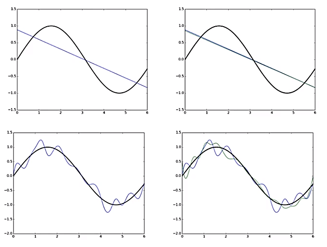
In the above graph, the black curve represents the true sinusoidal curve from which the data has come. The blue line in the first row of the picture represents the simple model trained over one random sample of training data.
If we take another subset of training data for the simple model, we’d get a different function (green line) because the model is learning different values for the parameters.
Let’s look at the case of a complex model. The blue polynomial curve represents the complex model trained on one random sample of training data, and the green curve represents the model trained on another random sample of training data. The same function trained on different data points is turning out to be very different.
- Simple models trained on different samples of data don’t differ much from each other. However, they’re very far from the true sinusoidal curve (underfitting).
- On the other hand, complex models trained on different subsets of data are very different from each other (overfitting).
Bias and Variance
In this section, we’ll formally define bias and variance and then see how our simple and complex models handle them.
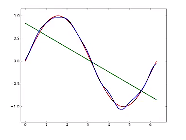
In the above figure,
- The green line represents the average value of predicted models for the simple approximation.
- The blue line represents the average value of predicted models for the complex approximation.
- The red line represents the true relationship.
Bias quantifies how far away the average of all the models fitted over all the possible training sets is from the true population line.

What bias captures is that over all the possible training sets, if the average function can’t capture anything close to the true relationship, then we can’t hope to get a good prediction interval.
From the above graph:
- We can see that for the simple model, the average value (green line) is very far from the true value (sinusoidal function). This means the simple model has high bias.
- On the other hand, the complex model (blue curve) has low bias.
Variance measures how much an estimate varies around its average. What variance captures is how much a model that we’re using for prediction—which we’ve fitted for a specific dataset—deviates from its expected fit over all the training datasets.
- It’s clear that the simple model has low variance, whereas the complex model has high variance.
In summary:
- Simple model: high bias, low variance
- Complex model: low bias, high variance
There’s always a trade-off between bias and variance because both contribute to the mean squared error loss.
Bias-Variance Trade-Off
In this section, we’ll analyze the effect of high bias and high variance on the test error. We’ve seen that the simple model failed miserably even on the training data; on the other hand, the complex model has done a pretty good job of fitting all the training points close to the true function. However, when it comes to testing, we’re interested in evaluating the model on unseen data.
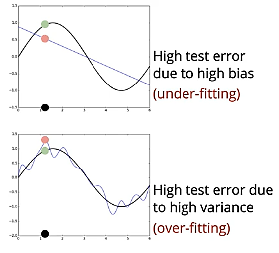
Consider a new point (x, y) (black point), which wasn’t seen during training, and the true output, which is shown as a green point. If we use the simple model for prediction, the predicted value would be far from the true output because of the simple model has a high bias.
Whereas, if we use the complex model, the value predicted by using the unseen data won’t be as close to the value we got from the training data. This is because the complex model focused too much on memorizing the patterns in the training data.
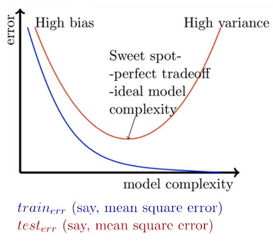
We’ve seen that as model complexity increases, training error reduces—but the complex model will have high variance because of overfitting. If we take the simple model, training and test error will both be high because of high bias. We want to get a model that balances both bias and variance such that training and test error would be at a minimum.
To solve this problem, we try to reach the sweet spot using the concept of regularization.
Overfitting in deep neural networks
In the previous sections, we’ve seen the bias-variance trade-off for our simple and complex models. In this section, we’ll discuss why we care about this bias-variance trade-off in the context of deep neural networks.
Deep neural networks are highly complex models (many parameters and many non-linearities) and they are easy to overfit (drive training error to zero); hence, we need some form of regularization.
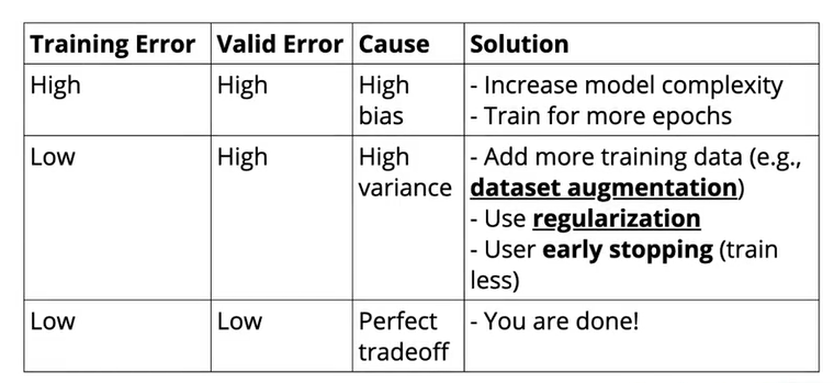
We’ve already seen that as model complexity increases, the bias of the model decreases and variance increases (and vice-versa). By using various regularization techniques, we can try to achieve low training and testing error so that we’re able to trade-off bias and variance perfectly.
For the remainder of this article, we’ll discuss the following regularization techniques:
- L2 Regularization
- Dataset Augmentation
- Early Stopping

L2 Regularization
Regularization has been used for decades prior to the advent of deep learning in linear models such as linear regression and logistic regression. Regularization techniques work by limiting the capacity of models—such as neural networks, linear regression, or logistic regression—by adding a parameter norm penalty Ω(θ) to the objective function. L2 regularization is also known as ridge regression or Tikhonov regularization.
Let’s assume that our objective is to minimize the squared error loss function, which is a function of theta θ, where θ indicates all the weights present in the network.
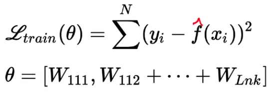
Instead of using the loss function L directly, we’ll add a regularization term Ω(θ) to the objective function.

When our training algorithm tries to minimize the regularized loss function, it will decrease both the original loss function and a regularization term. In the case of L2 regularization, the regularization term Ω(θ) is given as:
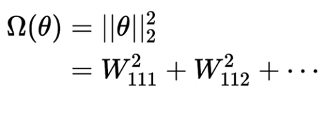
To minimize the regularized loss function, the algorithm should minimize both original the loss function plus the regularization term, which depends on the square of the weights. In effect, we’re adding the constraints to the original loss function, such that the weights of the network don’t grow too large. If the weights grow too large, the overall value of the regularized loss function would increase, meaning the network’s training loss would be more.
By adding the regularized term, we’re fooling the model such that it won’t drive the training error to zero, which in turn reduces the complexity of the model. Therefore, L2 regularization helps reduce the overfitting of data.
Dataset Augmentation
Dataset augmentation is a process of generating data artificially from the existing training data by doing minor changes like rotation, flips, adding blur to some pixels in the original image, or translations. Augmenting with more data will make it harder for the neural network to drive the training error to zero.
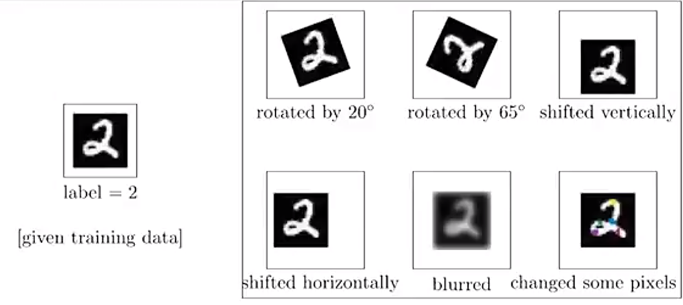
By generating more data, the network will have a better chance of performing better on the test data. Depending on the task at hand, we might use all the augmentation techniques and generate more training data.
To apply data augmentation, we can make use of the existing methods present in the frameworks like Keras, PyTorch. In Keras, we can use ImageDataGenerator to augment or create more data by doing transformations, and similarly, we can use the transforms class present in torchvision from PyTorch to augment data.
Early Stopping
The idea behind early stopping is that when we’re fitting a neural network on the training data and model is evaluated on the unseen data after each iteration. If the performance of the model on the validation data is not improving i.e…validation error is increasing or remaining the same for certain iterations, then there is no point in training the model further. This process of stopping model training before it reaches the lowest training error is known as early stopping.
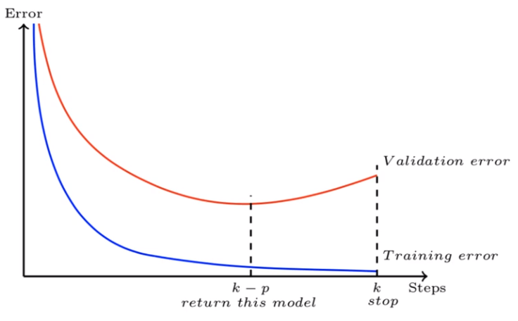
Let’s consider that we have set the patience of 5 epochs (i.e. the number of epochs to wait before early stop). For 5 epochs, we’ll monitor the validation error, and if it isn’t improving (either remains constant or increases) while the training error decreases, then we don’t want to train any further.
By using the early stopping technique, we’re making sure that the model doesn’t remember the patterns and noise present in the training data. Instead, we’re pushing it towards generalizing the training data.
Early stopping can be applied manually during the training process, or you can do even better by integrating these rules in your experiment through the hooks/callbacks provided in most common frameworks like Pytorch, Keras and TensorFlow.
Conclusion
In this post, we’ve discussed the need for regularization in deep neural networks. We then went on to formally define bias and variance for simple and complex models. After that, we looked at the trade-off between bias and variance as model complexity increases. We then discussed three regularization techniques to reduce neural network overfitting.
Continue Learning
If you are interested in learning more about Neural Networks, check out the Artificial Neural Networks by Abhishek and Pukhraj from Starttechacademy. Also, the course will be taught in the latest version of Tensorflow 2.0 (Keras backend). They also have a very good bundle on machine learning (Basics + Advanced) in both Python and R languages.
Recommended Reading
In my next post, we’ll discuss the convolution operation and how it relates to neural networks, leading to a network architecture known as a convolutional neural network. So make sure you follow me on Medium to get notified as soon as it drops.
Until then, Peace 🙂
NK.
Author Bio
Niranjan Kumar is Retail Risk Analyst at HSBC Analytics division. He is passionate about deep learning and AI. Apart from writing on Medium, he also writes for Marktechpost.com as a freelance data science writer. Check out his articles here.
You can connect with him on LinkedIn or follow him on Twitter for updates about upcoming articles on deep learning and machine learning.
Disclaimer — There might be some affiliate links in this post to relevant resources. You can purchase the bundle at the lowest price possible. I will receive a small commission if you purchase the course.

Comments 0 Responses