Linear regression is an algorithm that finds a linear relationship between a dependent variable and one or more independent variables. The dependent variable is also called label and independent variables are called features as well.
Linear regression is one of the most foundational algorithms for statistical and machine learning analysis.

PyTorch
PyTorch is an open source machine learning framework introduced by Facebook in 2016. PyTorch is based on the Torch library, and it’s a Python-based framework as well. Apart from its Python interface, PyTorch also has a C++ front end.
PyTorch is developed to provide high flexibility and speed during the implementation of deep neural networks. The most basic data type in PyTorch is a tensor, which is similar to NumPy ndarray.

Installing PyTorch
Before we proceed further with an implementation, we need to ensure that PyTorch is installed in our Python environment. Visit pytorch.org and select preferences and run the given command to install PyTorch locally.
Please ensure that you’ve have met the prerequisites, i.e. that you’ve already installed NumPy, depending on your package manager. Anaconda is a recommended package manager since it installs all dependencies. You can use the below link to create a command like below to install PyTorch on your machine:
Create Data
We want to create a linear regression project with PyTorch. First, we need a dataset to work on—we’ll be creating this dataset using Python.
But before creating the data set we must decide what data to create. For this, the fundamental mathematics behind linear regression will help. We know the equation of a line can be written as y = mx +c where m is slope of the line and c is y intercept.
While creating our dataset, we’ll use the above equation of the line and add some error. As you can see in the below code, we’re setting the value of m (slope of line) as 4 and setting the value of c (intercept of line) as 6.
We’re also introducing some impurity to the data with np.random.randn(91)*2 so that not all the data will fit properly on a line.
# importing library
import torch
from torch.autograd import Variable
import numpy as np
# Creating the dummy dataset
np.random.seed(42)
torch.manual_seed(42)
m = 4; c = 6
x = np.linspace(0, 11, 91)
y = m*x + c + np.random.randn(91)*2
x = x.reshape(-1, 1)
y = y.reshape(-1, 1)
Defining our model
PyTorch provides Python classes but not the functions to set up the model. The Python class extends the torch.nn.Module from the Torch library. PyTorch classes written in Python are executed by the class forward() method.
Model class is a subclass of the torch.nn.module. We’ll use a linear model with both the input and output dimension of one.
The model class name here is LinearRegressionModelClass. We’ve created two methods, __init__ and forward, inside the class.
# Defining a Model in PyTorch
class LinearRegressionModelClass(torch.nn.Module):
     def forward(self, x):
         y_prediction = self.model(x);
         return y_prediction;
     def __init__(self, in_dim, out_dim):
         super(LinearRegressionModelClass, self).__init__()
         self.model = torch.nn.Linear(in_dim, out_dim)
torch_model= LinearRegressionModelClass(in_dim=1, out_dim=1)
Training our model
We’ll be training the model with Mean Square Error as a loss function and Stochastic Gradient Descent as our optimizer. As you can see in the below code, MSELoss is the loss function and torch.optim.SGD is the optimizer. lr represents the learning rate and it’s used along with momentum. Momentum is something that can accelerate training, and the learning rate helps to converge the optimization process.
# Training the pytorch model
torch_optimizer = torch.optim.SGD(torch_model.parameters(), lr=0.012, momentum=0.82)
torch_cost = torch.nn.MSELoss()
torch_inputs = Variable(torch.from_numpy(x.astype('float32')))
torch_outputs = Variable(torch.from_numpy(y.astype('float32')))
for epocher in range(120):
    y_prediction = torch_model(torch_inputs)
    loss = torch_cost(y_prediction, torch_outputs)
    loss.backward()
    torch_optimizer.zero_grad();
    torch_optimizer.step()
    if ((epocher) % 12 == 0 ):
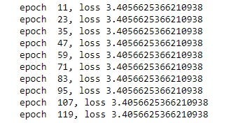
        print('epoch {}, loss {}'.format(epocher, loss.data))
Output


Prediction
After model training is completed, we can start making predictions using our model. Prediction is one of the most important steps—it allows us to check whether or not we’re getting correct results using the model. Here, we can do this by passing an input value of 6
Output:

Visualizing our results
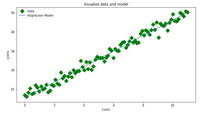
After the prediction, we also have options to visualize the model and its corresponding training data points in one plot. This will give us a better understanding of how the model is fitting on the data. We’re using matplotlib’s pyplot for this visualization.
# Visualize data and model
import matplotlib.pyplot as plt
%matplotlib inline
plt.figure(figsize=(11,6))
plt.title('Visualize data and model')
plt.xlabel('x-axis')
plt.ylabel('y-axis')
plt.plot(x, y, 'go', label='Data', marker='D', markersize=10)
plt.plot(x, torch_model.model.weight.item()*x+torch_model.model.bias.item(), label='Regression Model')
plt.legend();
plt.show()
Output:

Conclusion:
As per the graph, the model has correctly found the linear relationship between the dependent and independent variables.
The next step might be to try a linear regression model for a more complex linear equation that has multiple independent variables or features.
Feel free to change various parameters of model and play with the code.
Happy Machine Learning 🙂

Comments 0 Responses