“So unexpected was the hole that for several years computers analyzing ozone data had systematically thrown out the readings that should have pointed to its growth.” — New Scientist 31st March 1988
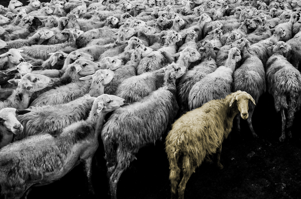
According to Wikipedia, an outlier is an observation point that is distant from other observations. This definition is vague because it doesn’t quantify the word “distant”. In this blog, we’ll try to understand the different interpretations of this “distant” notion. We will also look into the outlier detection and treatment techniques while seeing their impact on different types of machine learning models.
Outliers arise due to changes in system behavior, fraudulent behavior, human error, instrument error, or simply through natural deviations in populations. A sample may have been contaminated with elements from outside the population being examined.
Many machine learning models, like linear & logistic regression, are easily impacted by the outliers in the training data. Models like AdaBoost increase the weights of misclassified points on every iteration and therefore might put high weights on these outliers as they tend to be often misclassified. This can become an issue if that outlier is an error of some type, or if we want our model to generalize well and not care for extreme values.
To overcome this issue, we can either change the model or metric, or we can make some changes in the data and use the same models. For the analysis, we will look into House Prices Kaggle Data. All the codes for plots and implementation can be found on this GitHub Repository.
What do we mean by outliers?
Extreme values can be present in both dependent & independent variables, in the case of supervised learning methods.
These extreme values need not necessarily impact the model performance or accuracy, but when they do they are called “Influential” points.
Extreme Values in Independent Variables
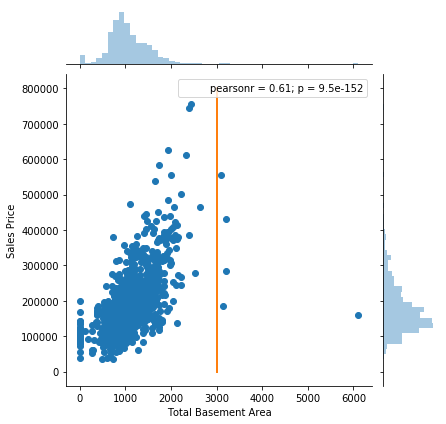
These are called points of “high leverage”. With a single predictor, an extreme value is simply one that is particularly high or low. With multiple predictors, extreme values may be particularly high or low for one or more predictors (univariate analysis — analysis of one variable at a time) or may be “unusual” combinations of predictor values (multivariate analysis)
In the following figure, all the points on the right-hand side of the orange line are leverage points.
Extreme Values in Target Variables
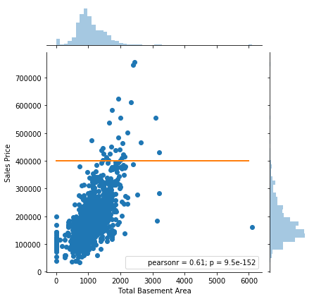
Regression — these extreme values are termed as “outliers”. They may or may not be influential points, which we will see later. In the following figure, all the points above the orange line can be classified as outliers.
Classification: Here, we have two types of extreme values:
1. Outliers: For example, in an image classification problem in which we’re trying to identify dogs/cats, one of the images in the training set has a gorilla (or any other category not part of the goal of the problem) by mistake. Here, the gorilla image is clearly noise. Detecting outliers here does not make sense because we already know which categories we want to focus on and which to discard
2. Novelties: Many times we’re dealing with novelties, and the problem is often called supervised anomaly detection. In this case, the goal is not to remove outliers or reduce their impact, but we are interested in detecting anomalies in new observations. Therefore we won’t be discussing it in this post. It is especially used for fraud detection in credit-card transactions, fake calls, etc.
All the points we have discussed above, including influential points, will become very clear once we visualize the following figure.
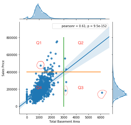
Our major focus will be outliers (extreme values in target variable for further investigation and treatment). We’ll see the impact of these extreme values on the model’s performance.
Common Methods for Detecting Outliers
When detecting outliers, we are either doing univariate analysis or multivariate analysis. When your linear model has a single predictor, then you can use univariate analysis. However, it can give misleading results if you use it for multiple predictors. One common way of performing outlier detection is to assume that the regular data come from a known distribution (e.g. data are Gaussian distributed). This assumption is discussed in the Z-Score method section below.
Box-Plot
The quickest and easiest way to identify outliers is by visualizing them using plots. If your dataset is not huge (approx. up to 10k observations & 100 features), I would highly recommend you build scatter plots & box-plots of variables. If there aren’t outliers, you’ll definitely gain some other insights like correlations, variability, or external factors like the impact of world war/recession on economic factors. However, this method is not recommended for high dimensional data where the power of visualization fails.
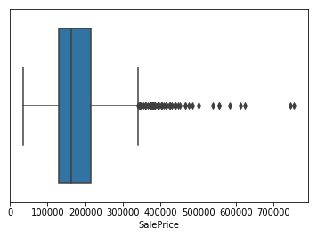
The box plot uses inter-quartile range to detect outliers. Here, we first determine the quartiles Q1 and Q3.
Interquartile range is given by, IQR = Q3 — Q1
Upper limit = Q3+1.5*IQR
Lower limit = Q1–1.5*IQR
Anything below the lower limit and above the upper limit is considered an outlier
Cook’s Distance
This is a multivariate approach for finding influential points. These points may or may not be outliers as explained above, but they have the power to influence the regression model. We will see their impact in the later part of the blog.
This method is used only for linear regression and therefore has a limited application. Cook’s distance measures the effect of deleting a given observation. It’s represents the sum of all the changes in the regression model when observation “i” is removed from it.

Here, p is the number of predictors and s² is the mean squared error of the regression model. There are different views regarding the cut-off values to use for spotting highly influential points. A rule of thumb is that D(i) > 4/n, can be good cut off for influential points.
R has the car (Companion to Applied Regression) package where you can directly find outliers using Cook’s distance. Implementation is provided in this R-Tutorial. Another similar approach is DFFITS, which you can see details of here.
Z-Score
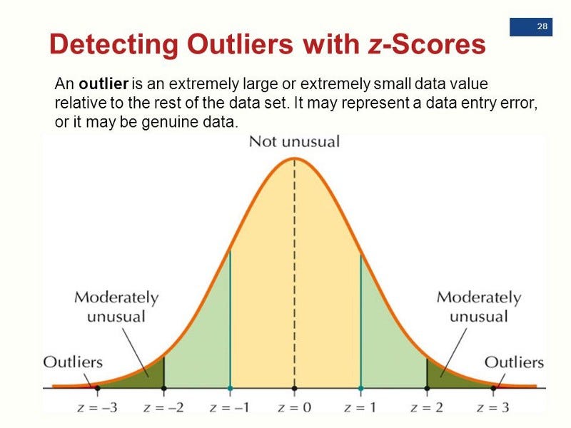
This method assumes that the variable has a Gaussian distribution. It represents the number of standard deviations an observation is away from the mean:

Here, we normally define outliers as points whose modulus of z-score is greater than a threshold value. This threshold value is usually greater than 2 (3 is a common value).
All the above methods are good for initial analysis of data, but they don’t have much value in multivariate settings or with high dimensional data. For such datasets, we have to use advanced methods like PCA, LOF (Local Outlier Factor) & HiCS: High Contrast Subspaces for Density-Based Outlier Ranking.
We won’t be discussing these methods in this blog, as they are beyond its scope. Our focus here is to see how various outlier treatment techniques affect the performance of models. You can read this blog for details on these methods.
Impact & Treatment of Outliers
The impact of outliers can be seen not only in predictive modeling but also in statistical tests where it reduces the power of tests. Most parametric statistics, like means, standard deviations, and correlations, and every statistic based on these, are highly sensitive to outliers. But in this post, we are focusing only on the impact of outliers in predictive modeling.
To Drop or Not to Drop
I believe dropping data is always a harsh step and should be taken only in extreme conditions when we’re very sure that the outlier is a measurement error, which we generally do not know. The data collection process is rarely provided. When we drop data, we lose information in terms of the variability in data. When we have too many observations and outliers are few, then we can think of dropping these observations.
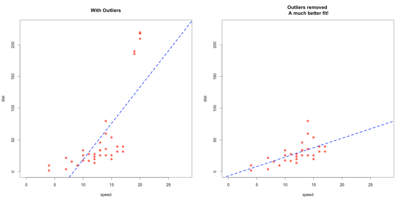
In the following example we can see that the slope of the regression line changes a lot in the presence of the extreme values at the top. Hence, it is reasonable to drop them and get a better fit & more general solution.
Other Data-Based Methods
- Winsorizing: This method involves setting the extreme values of an attribute to some specified value. For example, for a 90% Winsorization, the bottom 5% of values are set equal to the minimum value in the 5th percentile, while the upper 5% of values are set equal to the maximum value in the 95th percentile. This is more advanced than trimming where we just exclude the extreme values.
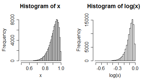
- Log-Scale Transformation: This method is often used to reduce the variability of data including outlying observation. Here, the y value is changed to log(y). It’s often preferred when the response variable follows exponential distribution or is right-skewed.
- However, it’s a controversial step and does not necessarily reduce the variance. For example, this answer beautifully captures all those cases.
- Poor example of transformation –
- Binning: This refers to dividing a list of continuous variables into groups. We do this to discover sets of patterns in continuous variables, which are difficult to analyze otherwise. But, it also leads to loss of information and loss of power.
Model-Based Methods
- Use a different model: Instead of linear models, we can use tree-based methods like Random Forests and Gradient Boosting techniques, which are less impacted by outliers. This answer clearly explains why tree based methods are robust to outliers.
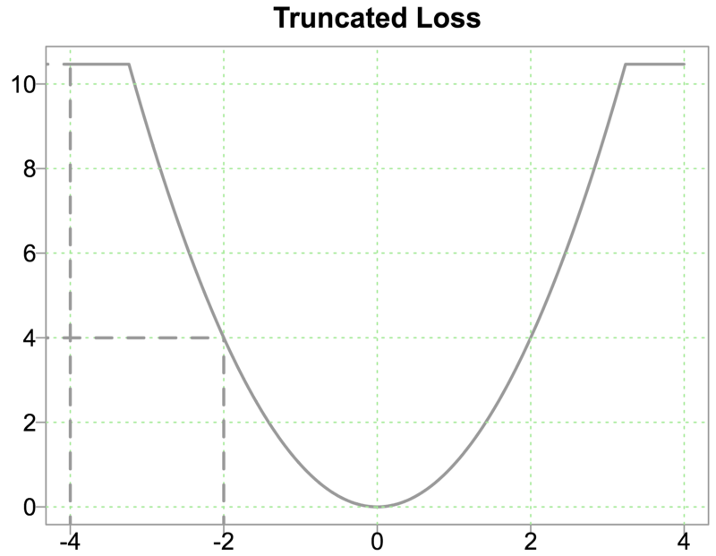
- Metrics: Use MAE instead of RMSE as a loss function. We can also use truncated loss:

Case Study Comparison
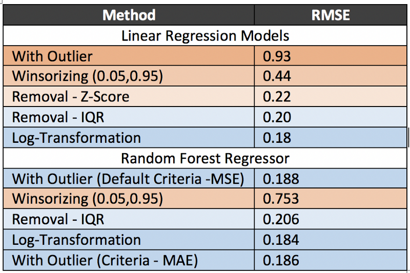
For this comparison, I chose only four important predictors (Overall Quality, MSubClass, Total Basement Area, Ground living area) out of total 80 predictors and tried to predict Sales Price using these predictors. The idea is to see how outliers affect linear & tree-based methods.
End Notes
- Since there are only 1400 total observation in the dataset, the impact of outliers is considerable on a linear regression model, as we can see from the RMSE scores of “With outliers” (0.93) and “Without outliers” (0.18) — a significant drop.
- For this dataset, the target variable is right skewed. Because of this, log-transformation works better than removing outliers. Hence we should always try to transform the data first rather than remove it. However, winsorizing is not as effective as compared to outlier removal. It might be because, by hard replacement, we are somehow introducing inaccuracies into the data.
- Clearly, Random Forest is not affected by outliers because after removing the outliers, RMSE increased. This might be the reason why changing the criteria from MSE to MAE did not help much (from 0.188 to 0.186). Even for this case, log-transformation turned out to be the winner: the reason being, the skewed nature of the target variable. After transformation, the data are becoming uniform and splitting is becoming better in the Random Forest.
From the above results, we can conclude that transformation techniques generally works better than dropping for improving the predictive accuracy of both linear & tree-based models. It is very important to treat outliers by either dropping or transforming them if you are using linear regression model.
If I have missed any important techniques for outliers treatment, I would love to hear about them in comments. Thank you for reading.
About Me: Graduated with Masters in Data Science at USF. Interested in working with cross-functional groups to derive insights from data, and apply Machine Learning knowledge to solve complicated data science problems. https://alviraswalin.wixsite.com/alvira
Check out my other blogs here!
LinkedIn: www.linkedin.com/in/alvira-swalin
References:
- The treatment methods have been taught by Yannet Interian at USF
- GitHub Repo for Codes
- Data For House Price Analysis
- Lesson on Distinction Between Outliers and High Leverage Observations
- Introduction to Outlier Detection Methods
- A Comprehensive Guide to Data Exploration
- Cook’s D Implementation in R
Discuss this post on Hacker News.

Comments 0 Responses