
Introduction
Experimental studies have shown that a few trees properly placed around buildings can reduce air conditioning needs by 30%, thus reducing energy consumption and bills.
Similarly, tree-based predictive modeling, implemented using decision trees, can increase a business’s profit by predicting, for example, what customers would prefer in future, thus helping them making informed decisions well in advance.
In the realm of machine learning, decision trees are among the most popular algorithms that can be used to solve both classification and regression tasks. In this article, we’ll study and implement a decision tree classification model.
Before we start the implementation, let’s go through some key concepts related to decision tree algorithms.
You may like to watch a video on Decision Tree from Scratch in Python
Key Concepts
Information Gain
Information gain is a measure of how much information a particular feature gives us about the class. More specifically, information gain measures the quality of a split and is a metric used during the training of a decision tree model.
In other words, information gain is a good measure for deciding the relevance of a feature in the data. For example, suppose that we’re building a decision tree for some data describing the customers of a business. Information gain is used to decide which of the feature of the customers are the most relevant, so they can be tested near the root of the tree.
Decision tree algorithms choose the highest information gain to split the tree; thus, we need to check all the features before splitting the tree at a particular node.
Entropy
Entropy is a measures of impurity or uncertainty in a given examples. Entropy can be a measure how unpredictable a dataset may be.
Gini coefficient
The Gini coefficient provides an index to measure inequality. Consider the example of comparing income distributions between similar societies in which everyone earns exactly the same amount. A value of 0 for the Gini coefficient means everybody is earning equally; and 1 means all the income of the country is earned by a single person.
Now that we have a grasp on some of the key terms and concepts in decision trees, let’s start implementing one!
Import the Libraries
Let’s start our implementation using Python and a Jupyter Notebook.
Once the Jupyter Notebook is up and running, the first thing we should do is import the necessary libraries.
We need to import:
- NumPy
- Pandas
- Seaborn
- train_test_split
- DecisionTreeClassifier
- metrics
To actually implement the decision tree classifier, we’re going to use scikit-learn, and we’ll import our DecisionTreeClassifier from sklearn.tree:
import numpy as np
import pandas as pd
import seaborn as sns
from sklearn.model_selection import train_test_split
from sklearn.tree import DecisionTreeClassifier
from sklearn import metrics
After importing the libraries, we need to load and check the data in Pandas.
Load the Data
Once the libraries are imported, our next step is to load the data, which is stored in the GitHub repository linked here. You can download the data and keep it in your local folder. After that, we can use the read_csv method of Pandas to load the data into a Pandas dataframe df, as shown below:
df = pd.read_csv(‘Decision-Tree-Classification-Data.csv’)
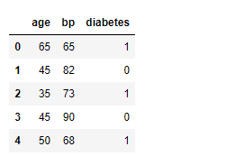
Also, in the snapshot of the data below, notice that the dataframe has three columns: age, bp (blood pressure), and diabetes. Here, age and bp are the features and diabetes is the label. We’re going to predict whether or not a person is suffering from diabetes using the person’s age and blood pressure value.
Data Pre-processing
Before feeding the data to the decision tree classifier, we need to do some pre-processing.
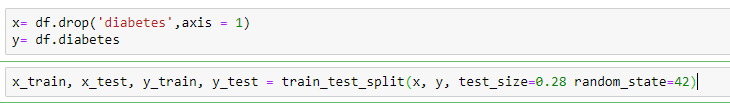
Here, we’ll create the x_train and y_train variables by taking them from the dataset and using the train_test_split function of scikit-learn to split the data into training and test sets.
Note that the test size of 0.28 indicates we’ve used 28% of the data for testing. random_state ensures reproducibility. For the output of train_test_split, we get x_train, x_test, y_train, and y_test values.
Training the Model
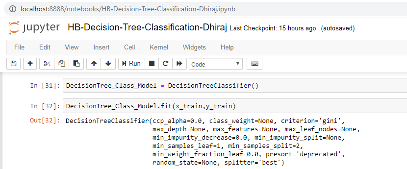
We’re going to use x_train and y_train, obtained above, to train our decision tree classifier. We’re using the fit method and passing the parameters as shown below.
Note that the output of this cell is describing a few parameters like criterion and max_depth for the model. All these parameters are configurable, and you’re free to tune them to match your requirements.
Predicting
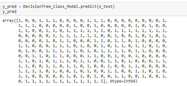
Once the model is trained, it’s ready to make predictions. We can use the predict method on the model and pass x_test as a parameter to get the output as y_pred.
Notice that the prediction output is an array of real numbers corresponding to the input array.
Evaluation
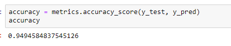
Finally, we need to check to see how well our model is performing on the test data. For this, we evaluate our model by finding the accuracy score produced by the model.
End notes
In this article, we discussed how to train and test a decision tree classifier. We also looked at how to pre-process and split the data into features (age and bp ) as variable x and labels as variable y (diabetic or not).
After that, we trained our model and then used it to run predictions. You can find the data used here.
Comments 0 Responses