Introduction
Do you remember climbing trees in your childhood? According to researchers, at the University of North Florida, climbing a tree can dramatically improve cognitive skills, including memory. Climbing trees can help children become more flexible in body and mind, while also developing strong spatial reasoning skills.
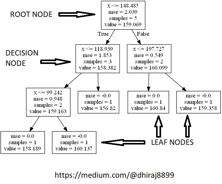
As it turns out, “trees” can also help machines learn. As illustrated below, decision trees are a type of algorithm that use a tree-like system of conditional control statements to create the machine learning model; hence, its name.

In the realm of machine learning, decision trees algorithm can be more suitable for regression problems than other common and popular algorithms. Below are the cases where you would likely prefer a decision tree over other regression algorithms:
- There are non-linear or complex relationships between features and labels
- You need a model that is easy to explain
Before we jump into an implementation of a decision tree for a regression problem, let’s define some key terms.
You may like to watch a video on Decision Tree from Scratch in Python
Decision trees: Key terms
- Root Node: The top-most decision node in a decision tree.
- Decision Node: A tree node or parent node that splits into one ore more child nodes is called a decision node.
- Leaf or Terminal Node: Bottom nodes that (generally speaking) don’t split any further.
- Splitting: Process of dividing a node into two or more child nodes.
- Pruning: The opposite process of splitting. Removing the child nodes of a decision node is called pruning.
Note that decision trees are typically plotted upside down, so that the root node is at the top and the leaf nodes are the bottom.
Decision tree algorithms can be applied to both regression and classification tasks; however, in this post we’ll work through a simple regression implementation using Python and scikit-learn.
Regression trees are used when the dependent variable is continuous.
For regression trees, the value of terminal nodes is the mean of the observations falling in that region. Therefore, if an unseen data point falls in that region, we predict using the mean value.

Now let’s start our implementation using Python and a Jupyter notebook.
Once the Jupyter notebook is up and running, the first thing we should do is import the necessary libraries.
Import the libraries
We need to import:
- NumPy
- Pandas
- DecisionTreeRegressor
- train_test_split
- r2_score
- mean squared error
- and Seaborn.
To actually implement the decision tree, we’re going to use scikit-learn, and we’ll import our DecisionTreeRegressor from sklearn.tree.
import numpy as np
import pandas as pd
from sklearn.tree import DecisionTreeRegressor
from sklearn.model_selection import train_test_split
from sklearn.metrics import r2_score,mean_squared_error
import seaborn as sns
Load the data
Once the libraries are imported, our next step is to load the data, stored here. You can download the data and keep it in your local folder. After that we can use the read_csv method of Pandas to load the data into a Pandas data frame df, as shown below.
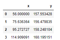
Also shown in the snapshot of data below, the data frame has two columns, x and y. Here x is the feature and y is the label. We’re going to predict y using x as an independent variable.
df = pd.read_csv(‘DT-Regression-Data.csv’)

Data pre-processing
Before feeding the data to the tree model, we need to do some pre-processing.
Here, we’ll create the x and y variables by taking them from the dataset and using the train_test_split function of scikit-learn to split the data into training and test sets.
We also need to reshape the values using the reshape method so that we can pass the data to train_test_split in the format required.
Note that the test size of 0.5 indicates we’ve used 50% of the data for testing. random_state ensures reproducibility. For the output of train_test_split we get x_train, x_test, y_train, and y_test values.
x = df.x
y = df.y
x = x.values.reshape(-1, 1)
y = y.values.reshape(-1, 1)
x_train, x_test, y_train, y_test = train_test_split(x, y, test_size=0.50, random_state=42)
Fit the model
We’re going to use x_train and y_train obtained above to train our decision tree regression model. We’re using the fit method and passing the parameters as shown below.
Note that the output of this cell is describing a large number of parameters like criteria, max depth, etc for the model. All these parameters are configurable, and you’re free to tune them to match your requirements.

Predict using the trained model
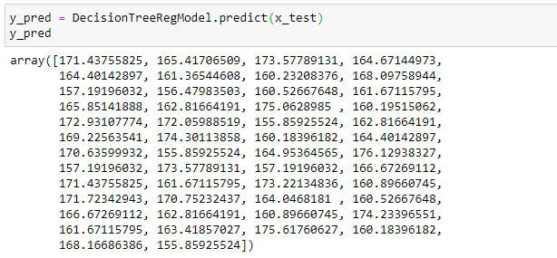
Once the model is trained, it’s ready to make predictions. We can use the predict method on the model and pass x_test as a parameter to get the output as y_pred.
Notice that the prediction output is an array of real numbers corresponding to the input array.

Model evaluation
Finally, we need to check to see how well our model is performing on the test data. For this, we evaluate our model by finding the root mean squared error produced by the model.
Mean squared error is a built in function, and we are using NumPy’s square root function (np.sqrt) on top of it to find the root mean squared error value.

End notes
In this article, we showed how to implement linear regression using a decision tree. We also looked at how to pre-process and split the data into features as variable x and labels as variable y.
After that, we trained our model and then used it to run predictions. You can find the data used here.

Congratulations on your newly-acquired skill set related to decision trees!
Happy learning!

Comments 0 Responses