This post is a part of a series about feature engineering techniques for machine learning with Python.
You can check out the rest of the articles:
- Hands-on with Feature Engineering Techniques: Broad Introduction.
- Hands-on with Feature Engineering Techniques: Variable Types.
- Hands-on with Feature Engineering Techniques: Common Issues in Datasets.
- Hands-on with Feature Engineering Techniques: Imputing Missing Values.
- Hands-on with Feature Engineering Techniques: Encoding Categorical Variables.
- Hands-on with Feature Engineering Techniques: Transforming Variables.
- Hands-on with Feature Engineering Techniques: Variable Discretization.
- Hands-on with Feature Engineering Techniques: Handling Outliers.
- Hands-on with Feature Engineering Techniques: Feature Scaling.
- Hands-on with Feature Engineering Techniques: Handling Date-time and Mixed Variables.
- Hands-on with Feature Engineering Techniques: Advanced Methods.
Welcome to the last of this series on feature engineering! In today’s article, we’ll explore some advanced feature engineering techniques across different tasks. Specifically, we’ll look at advanced categorical encoding, advanced outlier detection, automated feature engineering and more.
Advanced Categorical Encoding
We saw in a previous article some basic methods to encode categorical data. We’ll see in this section some other performant ways.
Make sure you’ve installed the Category Encoders library; if not, use the following commands in pip or conda:
Catboost Encoder
A CatBoost encoder is similar to target encoding, whose main objective is replacing the category with the mean target value for that category. Still, in CatBoost, the authors introduced the concept of time — the order of observations in the dataset.
In other words, for each row, the target probability is calculated only from the rows before it.
This process can cause overfitting, and to handle that the CatBoost encoder will repeat training numerous times on shuffled copies of the dataset, then we average the results.
Here is a code snippet with Python:
# import the pandas and catboost encoders libraries.
import pandas as pd
from category_encoders import CatBoostEncoder

# get you data.
data = pd.read_csv("yourData.csv")

# create the encoder.
encoder = CatBoostEncoder(return_df=True)

# fit and transform the data.
new_x_train = encoder.fit_transform(x_train, y_train)
new_x_test = encoder.transform(x_test, y_test)
And here is the detailed documentation:
Leave-one-out Encoder (LOO)
Leave-one-out encoding (LOO or LOOE) is an example of target-based encoding—it prevents target data leakage, unlike other target-based methods.
As its name suggests, the method consists of calculating the mean target of a given category k for observation j without using the corresponding target of j.
In other words, we calculate the per-category means with the typical target encoder, but we don’t include the current observation in that calculation.
Here is a sample code snippet for LOOE:
# import the pandas and Leave One Out encoders libraries.
import pandas as pd
from category_encoders import LeaveOneOutEncoder

# get you data.
data = pd.read_csv("yourData.csv")

# create the encoder.
encoder = LeaveOneOutEncoder(return_df=True)

# fit and transform the data.
new_x_train = encoder.fit_transform(x_train, y_train)
new_x_test = encoder.transform(x_test, y_test)
James-Stein Encoder
The James-Stein encoder is another example of a target-based encoder, which is defined for normal distributions.
James-Stein shrinks the average toward the overall average; it’s intended to improve the estimation of the category’s mean target by shrinking them towards a more median average.
Here is the formula to get the mean target for category k :

- n+/n is the estimation of the category’s mean target.
- y+/y is the central average of the mean target.
- B is a hyperparameter, representing the power of shrinking.
Here’s a code snippet:
# import the pandas and James Stein encoders libraries.
import pandas as pd
from category_encoders import JamesSteinEncoder

# get you data.
data = pd.read_csv("yourData.csv")

# create the encoder.
encoder = JamesSteinEncoder(return_df=True)

# fit and transform the data.
new_x_train = encoder.fit_transform(x_train, y_train)
new_x_test = encoder.transform(x_test, y_test)
Other Encoders
The Category Encoders library contains other powerful encoders you can experiment with, such as Helmert Coding and the M-estimate encoder—I definitely encourage you to take a look and test them yourself.
Advanced Missing Value Imputation
In a previous article we saw plenty of methods to handle missing data—today we’ll add other techniques to your toolkit for advanced imputation.
Iterative Imputation
Unlike the other imputation techniques, IterativeImputer is a Multivariate imputer that estimates each feature from all the other ones in a round-robin manner, while choosing how many repetitions the imputer will go through.
The imputer uses a strategy for imputing missing values by modeling each feature with missing values as a function of other features; therefore, the Imputer determines missing values by discovering patterns from its neighbors.
Using round-robin at each step:
- The algorithm chooses a feature as output y and all the other feature columns as inputs X.
- Train a regressor and fit it on (X, y) for known y.
- The regressor is used to predict the missing values of y.
- Repeat until the defined max_iteration is reached.
Here’s a code snippet:
# This estimator is still experimental, we need to explicitly require this experimental feature.
from sklearn.experimental import enable_iterative_imputer
from sklearn.impute import IterativeImputer

# create the imputer
imputer = IterativeImputer(random_state=22)

# fit the imputer to the train set
imputer.fit(train)

# transform the data
train_t = imputer.transform(train)
test_t = imputer.transform(test)
KNN Imputing
This imputation technique uses the famous KNN algorithm to predict the missing values from the neighbors. The idea is simple—any point value is approximated by the nearest point values of other variables.
For example, imagine we have a dataset of income, age, gender, and the income feature that has some missing values. For each missing income value, we look at the gender and the age of the person, then look for its K-nearest neighbors and get their corresponding income.
Here’s a code snippet:
# import the KNN imputer
from sklearn.impute import KNNImputer

# create the imputer with specefied number of neighbors (the K)
imputer = KNNImputer(n_neighbors=3)

# fit the imputer to the train set
imputer.fit(train)

# transform the data
train_t = imputer.transform(train)
test_t = imputer.transform(test)
Advanced Outlier detection
In an earlier post, we discussed an abundance of methods to handle and detect outliers, but we used only statistical measurements to denote the outliers. Here, we’ll explore some advanced algorithms to better detect these anomalies in datasets.
DBSCAN
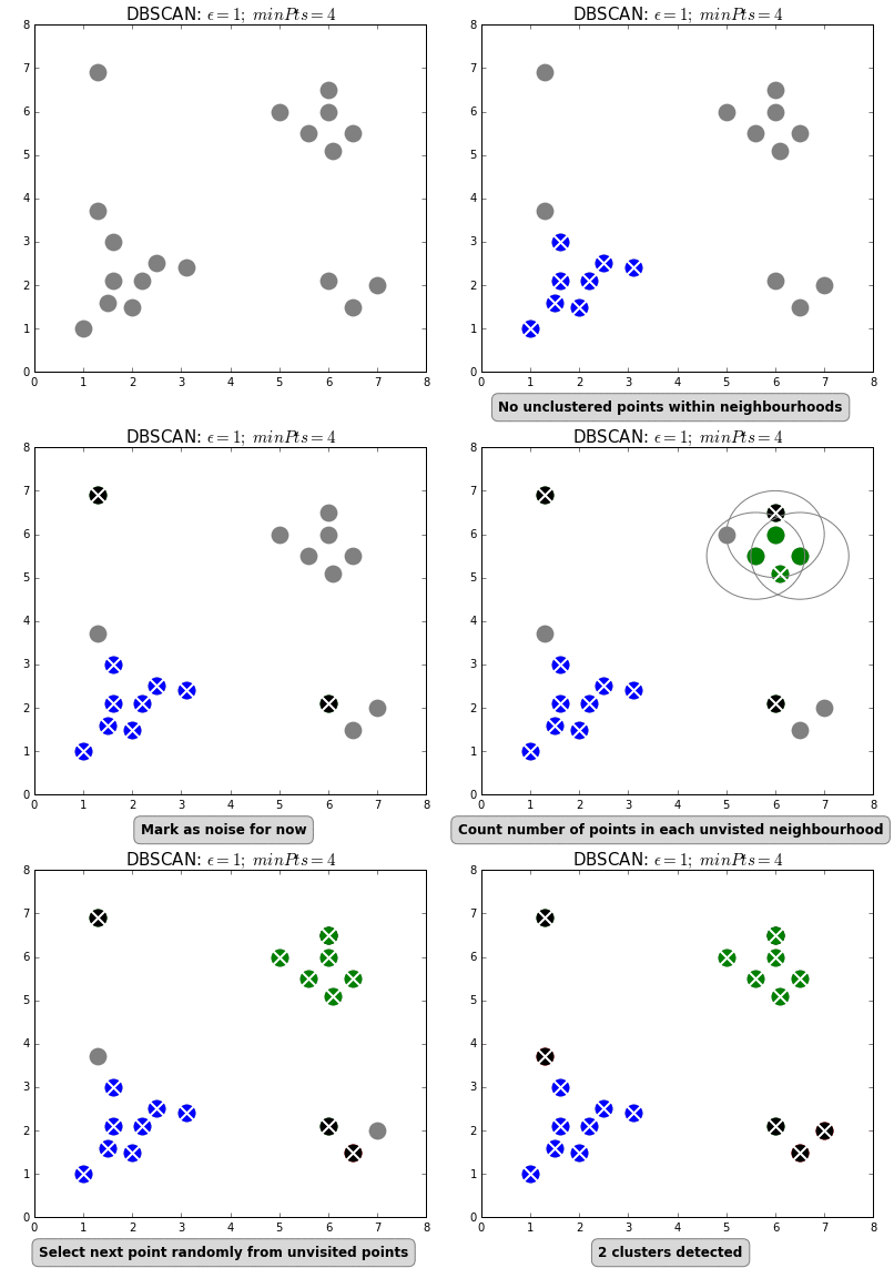
DBSCAN (Density-Based Spatial Clustering of Applications with Noise) is a clustering algorithm used to group points in the same clusters. It’s similar to K-means, but we do not specify the number of clusters in advance.

We use this algorithm to identify the points that do not belong to a cluster as outliers.
First we choose two hyperparameters:
- A positive number epsilon for the distances between points—it’s the maximum distance between two samples for one to be considered in the neighborhood of the other.
- A natural number min_samples, which serves as the number of samples in a neighborhood for a point to be considered as a core point.
Here is how the algorithm works:
- The algorithm randomly selects a point not assigned to a cluster.
- The algorithm determines if it belongs to a cluster by seeing if there are at least min_samples points around it within epsilon distance.
- The algorithm creates a cluster of this point with all other samples within epsilon distance to it.
- The algorithm then finds all points that are within epsilon distance of each point in that cluster and adds them to the same cluster.
- Finally, the algorithm finds all points that are within epsilon distance of all recently added points and adds these to the same cluster.
- Repeat steps 1–5
Now, after the algorithm finishes, all points not reachable from any other point are considered outliers.
Here is a great explanation and visualization playground tool to better understand the algorithm—you can manipulate the hyperparameter and test:
Here is a code snippet:
# import the libraries
from sklearn.cluster import DBSCAN
import pandas as pd

# read your data
data = pd.read_csv("yourData.csv")

# create the isolation forest
outlier_detection = DBSCAN(eps = 0.2, metric=”euclidean”, min_samples = 5, n_jobs = -1)

# fit and predict the outliers
outliers_cluster = outlier_detection.fit_predict(data)
Isolation Forests
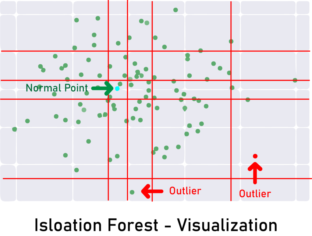
Unlike other outlier detection methods, an isolation forest explicitly searches and identifies outliers instead of the normal data points.
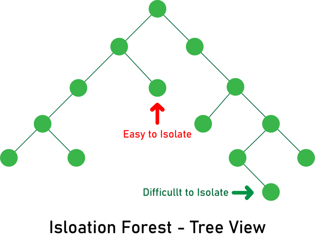
Isolation forest is built on the foundation of decision trees and uses tree ensemble methods, and as its name suggests, the algorithm examines how quickly a point can be isolated.
In simple words, the algorithm does random partitioning by randomly selecting a feature and then choosing a random split value.
A normal point will require more partitions to isolate, while outliers will be isolated quickly in the first splits.

Since outliers are less frequent than regular observations and lie further away from the regular observations in the feature space, with random partitioning they should be identified closer to the root of the tree. Here’s an illustration:

Here is a code snippet:
# import the libraries
from sklearn.ensemble import IsolationForest
import pandas as pd

# read your data
data = pd.read_csv("yourData.csv")

# create the isolation forest
outlier_detection = IsolationForest()

# fit and predict the outliers
outliers = outlier_detection.fit_predict(data)

#### OPTIONAL ###
# get index of outliers
outliers_index = np.where(outliers == -1, True, false)

# remove outliers from data.
data = data.loc[~(outliers_index, ]
Local Outlier Factor
Local outlier factor (LOF) measures the local variation of density of a given sample taking just its neighbors into consideration and not the global data distribution.
A point is marked as an outlier if the density around that point is significantly different from the density around its neighbors.
The algorithm follows these steps:
- Calculates the distances between a randomly selected point and every other point.
- Finds the farthest k closest point (k-th nearest-neighbor).
- Finds the other k closest points, like a normal KNN.
- Calculates the point density (local reachability density) using the inverse of the average distance between that point and its neighbors (the lower the density, the farther the point is from its neighbors).
- Calculates the LOF, which is essentially the average local reachability density of the neighbors divided by the point’s own local reachability density.
Here is the interpretation of the final LOF score:
- LOF(k) of 1 means similar density as neighbors.
- LOF(k) below 1 means higher density than neighbors (inlier).
- LOF(k) above 1 means lower density than neighbors (outlier).
Here’s a code snippet:
# import the libraries
from sklearn.neighbors import LocalOutlierFactor
import pandas as pd

# read your data
data = pd.read_csv("yourData.csv")

# create the isolation forest
outlier_detection = LocalOutlierFactor()

# fit and predict the outliers
outliers = outlier_detection.fit_predict(data)

#### OPTIONAL ###
# get index of outliers
outliers_index = np.where(outliers == -1, True, false)

# remove outliers from data.
data = data.loc[~(outliers_index, ]
Others
A great toolkit called PyOD for detecting outliers in multivariate data contains implementations of some advanced algorithms like PCA, variational auto-encoder, and the above-explained algorithms.
Here is how you can install it, and some resources to use it:
Automated Feature Engineering
Building and deploying machine learning models can often be a tedious process, from data loading and cleaning, feature engineering and feature selection, to training and validating the resulting models.
It would be nice if we could automate some of the tasks of the ML pipeline, especially the ones that require handcrafting like feature engineering tasks.
Hopefully, we can automate feature engineering, with a great concept called deep feature synthesis and an exceptional tool called Featuretools.
Deep Feature Synthesis
In December 2015 James Max Kanter and Kalyan Veeramachaneni proposed a Deep Feature Synthesis algorithm for automatically generating features for relational datasets.
You can read the original paper here, but here is the definition of the algorithm:
Featuretools
Featuretools is an open-source framework for implementing automated feature engineering.
It is a comprehensive tool intended to make the feature generation process fast-forward.
Featuretools has some components that you should be aware of in order to use:
- Deep Feature Synthesis: We already talked about this briefly above—the backbone of Featuretools.
- Entities: You can think of it as a Pandas dataframe—multiple entities result in an EntitySet.
- Feature primitives: The methods or operations that Deep Feature Synthesis applies to EntitySet—can be transformations or aggregations like count or average.
You can learn how to use Featuretools in Python from the following post:
Here is another great in-depth notebook to learn Featuretools:
Engineering Geospatial Data
We may often encounter geospatial features that are (most of the time) represented as longitude and latitude.
These features will influence your predictive model’s results by a large margin if they aren’t well-engineered.
Here’s an article that will show you how to work with this type of data — first by visualizing them to obtain valuable insights; then, exploring different methods you can use to extract and design new features that will improve your model.
Resampling Imbalanced Data
In classification, an issue can occur in datasets where the classes are not represented equally, which can cause huge problems for some algorithms.
Here is an article that explores a technique called resampling to engineer and reduce this effect on our machine learning algorithms.
Conclusion
We saw plenty of innovative, advanced methods you can use in your feature engineering toolkit. I’d encourage you to experiment with different methods and techniques to get the best results.
I hope you enjoyed this series as much as I did, and that you’ve learned at least a technique (or several) to apply in your machine learning and data science projects.
In machine learning, you have to test, combine, and innovate approaches to see what works better for your problem. There is no magic code snippet that can give the best results all the time — instead, this is an art that requires creativity.

Comments 0 Responses