Convolutional Neural Networks (CNNs): Core Concepts Applied

In this tutorial, we’ll work through the core concepts of convolutional neural networks (CNNs). To do this, we’ll use a common dataset — the MNIST dataset—and a standard deep learning task—image classification

The goal here is to walk through an example that will illustrate the processes involved in building a convolutional neural network. The skills you will learn here can easily be transferred to a separate dataset.

So let’s go deeper…pun intended.

Setup

In this step, we need to import Keras and other packages that we’re going to use in building our CNN. Import the following packages:

• Sequential is used to initialize the neural network.
• Conv2D is used to make the convolutional network work with images.
• MaxPooling2D is used to add the pooling layers.
• Flatten is the function that converts the pooled feature map to a single column, which is then passed to the fully connected layer.
• Dense adds the fully connected layer to the neural network.
• Reshape is used to change the shape of the input array

Import the Dataset

Next, we’ll import the mnist dataset from Keras. We load in the training set and the testing set. We have to scale our data so that it will be compatible with our network. In this case, we scale the images by dividing them by 255. This will ensure that the array values are numbers between 0 and 1.

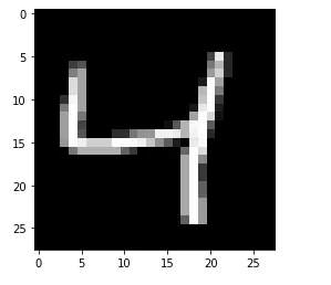
Visualize a digit

We can visualize a single digit using Matplotlib. This is important so that we can see a sample of what the digits in the dataset look like.

Setup

In this step, we need to import Keras and other packages that we’re going to use in building the CNN. Import the following packages:

• Sequential is used to initialize the neural network.
• Conv2D is used to make the convolutional network that deals with the images.
• MaxPooling2D layer is used to add the pooling layers.
• Flatten is the function that converts the pooled feature map to a single column that is passed to the fully connected layer.
• Dense adds the fully connected layer to the neural network.
• Reshape for changing the shape of the input array

Import the Dataset

Next, we’ll import the mnist dataset from Keras. We load in the training set and the testing set. We’ve seen previously that we have to scale our data. In this case, we scale the images by dividing by 255. This will ensure that the array values are numbers between 0 and 1.

Visualize a Number

We can visualize a single digit using Matplotlib.

Building the Network

Before we start building the network, let’s confirm the shape of the training data. This is important because the shape will be needed by the convolution layer. We’ll use this shape later to reshape the size of the input data.

We kick off by initializing the sequential model. Then we pass in our layers as a list. The first layer is the reshape layer for changing the shape of the input data. We already know that each image has a size of 28 by 28. We also pass 1 to the reshape layer to ensure that the input data has a single color channel.

Next, we create the convolution layer. This layer takes in a couple of parameters:

• filters — the number of output filters in the convolution, i.e the number of feature detectors. 32 is a common number of feature detectors used.
• kernel_size — the dimensions of the feature detector matrix. This is the width and height of the convolution window.
• input_shape — the shape of the input data. Since we included a reshape layer, we don’t need to pass this.
• activation — the activation function to be uses. The ReLu activation function is a common choice.

The next item on the list is to add the pooling layer. In this step, the size of the feature map is reduced by taking the maximum value during the pooling process. 2 by 2 is a commonly-used pool size. This will reduce the size of the feature map while maintaining the most important features needed to identify the digits.

After that, we flatten the feature maps. This will convert the feature maps into a single column.

The results obtained above are then passed to the dense layer. The parameters passed to this layer are the number of neurons and the activation function. In this case, those are 128 and ReLu, respectively.

Finally, we created our output layer. 10 is used here, because our dataset has 10 classes. We’ll use the softmax activation function because classes are mutually exclusive—an image can’t be, for example, classified as numbers 0 and 1 at the same time. If the case was otherwise, we’d use the sigmoid activation function.

Compiling the Network

We now need to apply gradient descent to the number. This is done at the compile stage. We pass the following parameters:

• optimizer — the type of gradient descent to use; in this case, we’ll use stochastic gradient descent
• loss — the cost function to use. We use sparse_categorical_crossentropy because the classes are integer-encoded. Had we performed one-hot encoding, we’d have to use the categorical cross-entropy loss function.
• metrics — the evaluation metrics to monitor; in this case, accuracy

Fitting the CNN

Next, we fit the training set to the network. epochs is the number of rounds the data will pass through the network. validation_data is the test dataset that will be used to evalutate the performance of the model during training.

Evaluating the Network

We can now check the performance of the network. We do so using the evaluate function, passing in the test set. The first item in the result produced is the loss, and the second is the accuracy.

Checking the Predictions

Let’s now see if our network is able to correctly identify a digit. We kick off by making predictions:

For example, let’s check the digit at index 2 in the test set.

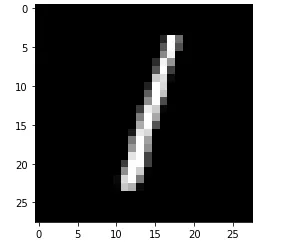
This is clearly the digit one. Let’s compare that with the prediction made for digit 1.

From the predictions below, we can see that the digit 1 — at index 1 in the prediction array— has the highest prediction.

0.00077352 — digit 0 prediction

99.63969 — digit 1 prediction

0.07214971 — digit 2 prediction

0.03056707 — digit 3 prediction

0.00606834 — digit 4 prediction

0.00301009 — digit 5 prediction

0.02507676 — digit 6 prediction

0.11558129 — digit 7 prediction

0.10332227 — digit 8 prediction

0.00378496 — digit 9 prediction

We can check another prediction by plotting the digit at index 0 in the testing set. Let’s try number 7.

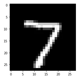
Next, we’ll look at the prediction at index 0 to see if it’s also number 7. Clearly, 7 has the highest prediction.

Conclusion

Well done for making it this far! In this article, we’ve used CNN core concepts to develop a working convolutional neural network. We have seen the steps you’ll need to take, and we’ve evaluated our trained model. Now you can try this out with a different dataset to see if you can reproduce the network we built here.