Building an Image Recognition Model for Mobile using Depthwise Convolutions

Deep Learning algorithms are excellent at solving very complex problems, including Image Recognition, Object Detection, Language Translation, Speech Recognition, and Synthesis, and include many more applications, such as Generative Models.

However, deep learning is extremely compute intensive—it’s generally only viable through acceleration by powerful general-purpose GPUs, especially from Nvidia.

Unfortunately, mobile devices have very limited compute capacity; hence, most architectures that have been very successful on desktop computers and servers cannot be directly deployed to mobile devices.

However, a number of techniques exist for making deep learning models efficient enough for mobile devices. Chief of these is “Depthwise Convolutions.”

Depthwise convolutions are the foundation of the popular Google MobileNet papers. They also formed the basis of Xception by Francois Collet.

They’re very similar to standard convolutions but are different in a few specific ways that make them extremely efficient. In this tutorial, I’ll explain how they differ from regular convolutions and how to apply them in building an image recognition model suitable for deployment on mobile devices.

How Depthwise Convolutions Work

Standard Convolutions

To fully appreciate the efficiency of depthwise convolutions, I’ll first explain how standard convolutions work.

Below is a diagram I drew up to illustrate standard convolutions.

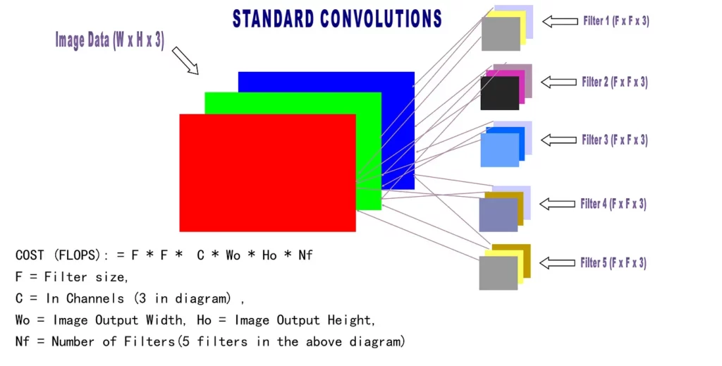
Convolutions are used to detect fixed-size features in an image. Color images are made up of pixels arranged in a stack of three color channels: RED, GREEN and BLUE (RGB). To extract useful features from the image, a convolution is composed of N filters, with each filter representing a feature. Hence, a convolution with 32 filters will detect 32 features in an image. Each filter has a fixed size—common filter sizes are 1 x 1, 2 x 2 , 3 x 3, 4 x 4, and 5 x 5.

In the diagram above, we have a W X H X 3 image. We apply a convolution with 5 filters to detect 5 distinct features in the image. Our filter is F x F in size, and since our image has 3 channels, the filter size will effectively be F x F x 3.

The result of this convolution will be Wo x Ho x 5. Hence, the computational cost in Multiply Adds for this will be: F * F * 3 * Wo * Ho * 5

A 3 x 3 convolution with 128 filters, operating on an input of size 112 x 112 x 64, with a stride of 1 and padding of 1 will have a cost of: 3 * 3 * 64 * 112 * 112 * 128 = 924 Million Multiply Adds

Generally, the formula for calculating the cost of a convolution is:

FILTER DIM * Image Output DIM

Since FILTER DIM = F X F X C

and Image Output DIM = Wo X Ho X Nf

The formula for standard convolutions is: F * F * C * Wo * Ho * Nf

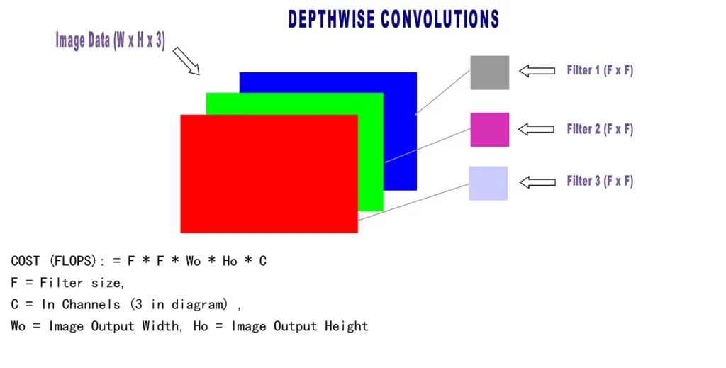
Depthwise Convolutions

Depthwise Convolutions operate in similar fashion but with the following differences:

1. Each filter operates on a single channel

2. The number of filters is equal to the number of image input channels

The two constraints above imply that every filter operates on each channel separately. Hence, an image with 3 channels will need 3 filters, and each filter will have an effective size of F X F. For example, 2 X 2 X 3 filters in the standard convolution will be simply 2 x 2 in depthwise convolutions.

In depthwise convolutions,

FILTER DIM = F X F

Output DIM = Wo X Ho X C

According to the formula, COST = FILTER DIM * Image Output DIM

The formula for depthwise convolutions is: F * F * Wo * Ho * C

Hence, a 3 x 3 depthwise convolution operating on a input of size 112 x 112 x 128, with a stride of 1 and padding of 1 will have a cost of: 3 * 3 * 112 * 112 * 128 = 14.45 Million Multiply Adds

As you can see, for the same input size, stride, and padding, a standard convolution has a cost of 924 million multiply adds, while depthwise convolutions have a cost of 14.45 million multiply adds.

That’s an astonishing difference!

Usually, to capture cross-channel dependencies, standard 1 x 1 convolutions are applied before or after depthwise convolutions. However, since a 1 x 1 convolution is 9 times less expensive than a 3 x 3 convolution, the computational gains are still huge.

Implementing Google MobileNetV2

To illustrate how to use depthwise convolutions in practice, I’ll actually create a Keras implementation of the MobileNetV2 paper titled, “Inverted Residuals and Linear BottleNecks: Mobile Networks for Classification, Detection and Segmentation”, which you can find below:

The core of this model is the Linear Bottleneck module, it is structured as 1 x 1 Conv — 3 x 3 DepthwiseConv — 1 x 1 Conv, as seen in the code below.

import keras
from keras.layers import *
from keras.models import *

#The Linear Bottleneck increases the number of channels going into the depthwise convs
def LinearBottleNeck(x,in_channels,out_channnels,stride,expansion):

    #Expand the input channels
    out = Conv2D(in_channels*expansion,kernel_size=1,strides=1,padding="same",use_bias=False)(x)
    out = BatchNormalization()(out)
    out = Activation(relu6)(out)

    #perform 3 x 3 depthwise conv
    out = DepthwiseConv2D(kernel_size=3,strides=stride,padding="same",use_bias=False)(out)
    out = BatchNormalization()(out)
    out = Activation(relu6)(out)

    #Reduce the output channels to conserve computation
    out = Conv2D(out_channnels,kernel_size=1,strides=1,padding="same",use_bias=False)(out)
    out = BatchNormalization()(out)

    #Perform resnet-like addition if input image and output image are same dimesions
    if stride == 1 and in_channels == out_channnels:
        out = add([out,x])
    return out

The basic intuition behind this structure is to use a 1 x 1 convolution to project the input to have more channels; hence, our 3 x 3 depthwise convolution is able to detect more features. To reduce computational cost, another 1 x 1 convolution is used to reduce the number of output channels.

You might notice the relu6 function above—this is used to threshold activations to have a maximum value of 6. The function is defined below:

#Relu6 is the standard relu with the maximum thresholded to 6
def relu6(x):
    return K.relu(x,max_value=6)

The linear bottleneck is then stacked together to form the entire network. See the full model below:

def MobileNetV2(input_shape,num_classes=1000,multiplier=1.0):

    images = Input(shape=input_shape)

    net = Conv2D(int(32*multiplier),kernel_size=3,strides=2,padding="same",use_bias=False)(images)
    net = BatchNormalization()(net)
    net = Activation("relu")(net)

    channels = [16] + [24] * 2 + [32] * 3 + [64] * 4 + [96] * 3 + [160] * 3 + [320]
    strides = [1] + [2,1] + [2,1,1] + [2,1,1,1] + [1] * 3 + [2,1,1] + [1]
    expansions = [1] + [6] * 16


    in_channels = int(32 * multiplier)

    #Stack up multiple LinearBottlenecks
    for out_channels, stride, expansion in zip(channels,strides,expansions):
        out_channels = int(out_channels * multiplier)

        net = LinearBottleNeck(net,in_channels,out_channels,stride,expansion)
        in_channels = out_channels

    #Final number of channels must be at least 1280
    final_channels = int(1280 * multiplier) if multiplier > 1.0 else 1280

    #Expand the output channels
    net = Conv2D(final_channels,kernel_size=1,padding="same",use_bias=False)(net)
    net = BatchNormalization()(net)
    net = Activation(relu6)(net)

    #Final Classification is by 1 x 1 Conv
    net = AveragePooling2D(pool_size=(7,7))(net)
    net = Conv2D(num_classes,kernel_size=1,use_bias=False)(net)
    net = Flatten()(net)
    net = Activation("softmax")(net)

    return Model(inputs=images,outputs=net)

In the above, the multiplier set to 1.0 is used to scale the performance of the network.

The network above has a computational cost of 300 million multiply adds while boasting a top1 accuracy of 71.7% on ImageNet. Increasing the multiplier to 1.4 increases the cost to 585 million multiply adds while increasing accuracy to 74.7%.

Conclusion

Depthwise convolutions are efficient, and they achieve very high accuracy on Image Classification tasks while incurring minimal computational cost. Their use has also been extended to Object Detection, Image Segmentation and Neural Machine Translation (Kaiser et al, 2017, see below).

Generally speaking, standard convolutions still outperform depthwise convolutions. However, for mobile devices with limited compute capacity, depthwise convolutions are the best fit.

If you enjoyed reading this, give some CLAPS! You can always reach me on twitter at @johnolafenwa

Discuss this post on Hacker News and Reddit.