Introduction to Transfer Functions
This write up is an excerpt from my recent research on transfer functions and machine learning operations. Throughout this post, I’ll basically be establishing the core principles of these two different concepts, and examine their relationship to each other.
I have always understood machine learning algorithms as a simple relationship between variable X and Y, where X is the input data and Y is the learning outcome. The general polynomial relationship between X and Y is bounded by the following function:

In a case where we have just a single input pattern to learn from, we can model the data using polymeric regression. All we need to control is the value n (the order of polynomial). When n is 2, we can say the equation above reduces to a quadratic equation, given below:

What’s next is to feed in the data into the algorithm, and the algorithm will find the best value for A, B, and C depending on the problem at hand, be it classification or regression.
But what if we have a problem with multiple inputs or features—how do we model this mathematically? We do have the equation below:

The above linear equation implies that every machine learning model follows similar patterns mathematically. A model totally replicates data if and only if it has been able to optimally determine the values of the feature parameter and the best value of the bias vector that best represents the data.
In essence, a machine learning model is either a linear or non-linear function that maps an input feature to its corresponding output result.

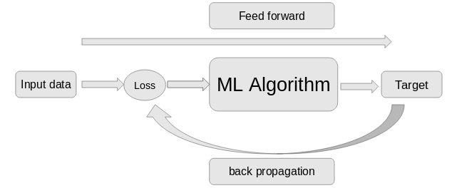
The diagram above clearly explains the machine learning workflow—how a model learns from its input data to arrive at the target. Optimal performance of the modeled data can only be achieved if there’s a good correlation or linkage point between the input data parameters and its target value. If not, there will be difficulty in the learning process.
More specifically, a model can be called “good” if (and only if) there are patterns to learn, and said model was able to figure it out. It’s a bad model if (and only if) there are no patterns due to an irregular correlation between input data points and the output target.
I will leave you with this phrase—your model is as good as the relevance of your data points to the target.
Concept of transfer functions
A transfer function is a system/mathematical function that models the output of a system with respect to its corresponding input. It’s mostly referred to as an electrical term used in modeling electrical devices of certain characteristics.
In plain terms, for instance, desirable electronic/electrical systems are modeled mathematically using transfer functions in order to be able to arrive at the desirable output signal. In the long run, the physically modeled system is represented by a passive device of known characteristics/responses (like capacitors, resistors, inductors). This is finally reordered to provide the overall input-output system response we desire.
A machine learning problem can be most simply modeled as a single input to a single output (SISO). We can also have more complex models, with multiple inputs to multiple outputs (MIMO). Just as we have these systems in machine learning, we also see them in transfer functions.
Consider fundamental machine learning problems like classification or regression—basically multiple input to single output (MISO) systems. Can we also say we have such systems in transfer functions? Yes, this is possible. But let’s look more closely at SISOs, which are the basis of transfer functions.
Transfer functions explained
Transfer functions are mathematical functions that models the output y(t) (a time varying function) of a system with respect to input x(t). Here, it’s important to note that the input has a notation that denotes its pattern, so does the output. A transfer function basically tries to find the mathematical relationship between the input pattern and the desirable pattern (output).
Let’s work through a quick example to see this in practice. For instance, if you have a system (desirable) whose characteristic equation is given by y(t) and another system of characteristic equation x(t), and you want to arrive at y(t) from x(t), you would need a transfer function to relate the two systems:

x(t) and y(t) are two different parameters with different characteristics, but we believe there’s a relationship between them.
A transfer function can come in handy to relate these two separate systems, such that we can get y(t) using the transfer function (or the reverse). Transfer functions are basically solutions represented in the frequency domain. The frequency domain refers to the analytic space in which mathematical functions or signals are conveyed in terms of frequency, rather than time.
Time domain functions are mathematical functions derived with respect to time, just like x(t) and y(t). Similarly, frequency domain functions are functions expressed with respect to frequency.
We often convert to a frequency domain because, in the frequency domain space, problems are easily solved, compared to using the time domain. In the time domain, variations of amplitude are over emphasized, but in the frequency domain, the response of the system is represented as a function of frequency.
Most systems you want to model would definitely have to be represented as a time domain system (that is, a system that varies with respect to time). But arriving at the desirable solution can be difficult when solving with respect to time.
Fortunately, solving such a system in the frequency domain is easier than solving the same system in the time domain. We therefore need to be able to represent such systems in the frequency domain and then convert the solution back to time domain.
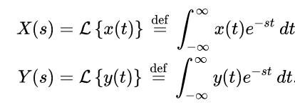
One of the ways we can do this is through the use of Laplace transforms. The Laplacian transform of function x(t) to a frequency domain function X(s) is defined below. For input function x(t) and output function y(t) we do have.


The question we might want to ask here is, what is, s? ‘S’ is basically called the ‘s-plane’, on which Laplace transforms are graphed. It’s a complex plane with σ representing the value on the real line and ω representing the value on the j-axis (imaginary axis).

The transfer function H(s), with respect to X(s) and Y(s), is denoted as:


Using symbolab, the solution to x(t) and y(t) assuming all initial conditions to be zero, is given as:


We can say that a time varying solution model that relates x(t) and y(t) is simply given as:

Comparison and relationship
Transfer functions basically work for any time varying system—it could be any form of signal representation—and are used as a signal processing technique for image processing and other computer vision applications. It works as long as you’re able to model the system accurately.
Essentially, they both figure out patterns between input data points and output data points. They both have their optimization approaches, but different techniques.
Transfer functions utilize the frequency domain technique in figuring out the pattern; and machine learning models utilizes activation functions and primitive metrics in learning patterns.
Conclusion
As we conclude, there’s something you should take note of: a machine learning model does process a set of inputs with respect to a target output, but transfer functions allow us to model a single input or more to an output.
Here, I’m emphasizing a single input/single output situation because we can actually have an optimized transfer function that mimics the pattern in a single feature with respect to the desired output.
Every input feature has patterns in its data representation that can be converted into a time domain function, which helps explain the pattern of that singular feature. If we have this, then we can model the relationship between that singular input with respect to the desired result or pattern (a time varying function)
Thanks for reading.
Reference
- https://deepai.org/machine-learning-glossary-and-terms/frequency-domain
- https://www.researchgate.net/post/What_is_the_difference_between_Time_domain_and_frequency_domain10
- http://tutorial.math.lamar.edu/Classes/DE/Laplace_Table.aspx
- https://intellipaat.com/community/16651/neural-network-activation-function-vs-transfer-function
- https://www.allaboutcircuits.com/textbook/semiconductors/chpt-1/active-versus-passive-devices/

Comments 0 Responses