
When training an artificial neural network (ANN), there are a number of hyperparameters to select, including the number of hidden layers, the number of hidden neurons per each hidden layer, the learning rate, and a regularization parameter. Creating the optimal mix from such hyperparameters is a challenging task.
A question commonly asked by beginners to ANNs is whether it’s possible to select an optimal architecture. A neural network’s architecture can simply be defined as the number of layers (especially the hidden ones) and the number of hidden neurons within these layers.
In one of my previous tutorials titled “Deduce the Number of Layers and Neurons for ANN” available at DataCamp, I presented an approach to handle this question theoretically.
This tutorial is going to ensure that the theory works by training an ANN created in Python based on the number of (theoretically) selected hidden layers/neurons and see whether things are working as expected or not.
There are many hyperparameters to optimize when working with ANNs. Being sure that the selected number of hidden layers and hidden neurons is the optimal choice lets you remove them from the hyperparameter optimization search space. As a result, less hyperparameters end up needing to be optimized.
The steps we’ll follow for each example are:
- Investigate the problem to decide, theoretically, the best number of hidden layers and hidden neurons (as discussed in the previous tutorial).
- Implement an ANN classifier in Python based on these selected numbers.
- Train the ANN to ensure whether the problem is solved optimally using these selected numbers (i.e. number of hidden layers and hidden neurons).
It’s very important to notice that the explanation in that tutorial works 100% for simple problems (i.e. when data is visualized in 2D). By increasing the number of variables representing each data sample, the process will not be as straightforward.
The objective here is to help us know the procedure we should follow to determine the best number of hidden layers/neurons. For complex problems, trial and error is still a good option to select hyperparameter values.
Example 1
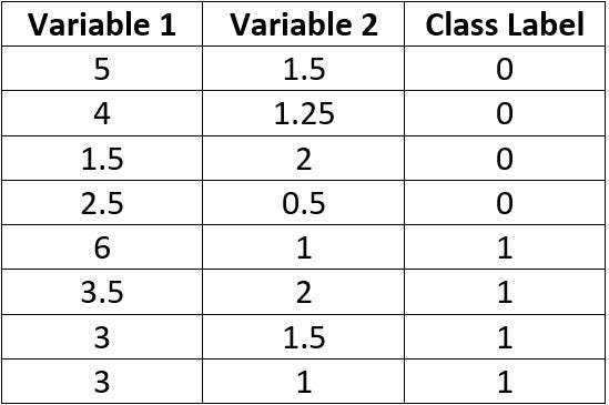
The first binary classification example has the samples and class labels given in the below table. We want to build an ANN to optimally classify the samples.
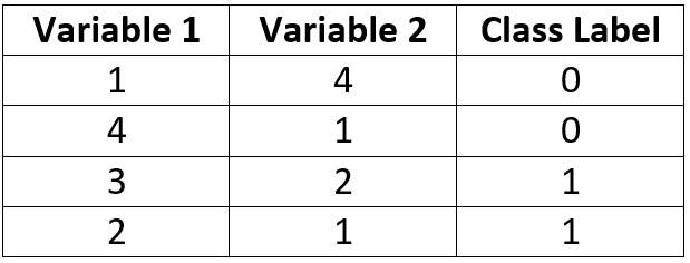
In designing an ANN architecture, we can start by selecting the number of neurons in the input and output layers. This example uses 2 variables as inputs for each sample, thus there will be 2 input neurons. Because this example is a binary classification problem, we can just use 1 output neuron. For more than 2 classes, we’d need to create an output neuron for each class.
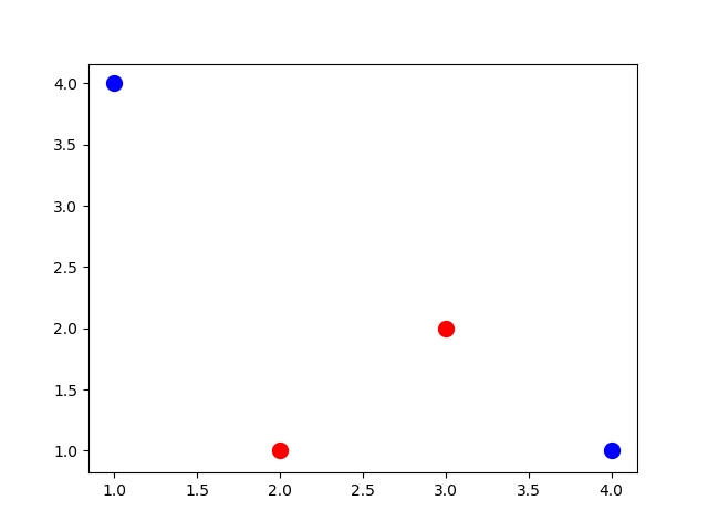
According to the previous tutorial, the first step for deducing the best number of hidden layers and neurons is to visualize the samples in a 2D graph. Below is the Python code used for plotting the data. The data inputs are stored in the input_data variable, while the output_data variable stores their outputs. All data samples are represented as dots in the plot. The blue color is assigned to samples from the first class, while the other samples are assigned the red color.
import numpy
import matplotlib.pyplot

input_data = numpy.array([[1, 4],
                          [4, 1],
                          [3, 2],
                          [2, 1]])
output_data = numpy.array([0, 0, 1, 1])

matplotlib.pyplot.scatter(input_data[:2, 0], input_data[:2, 1], color='blue', linewidths=5)
matplotlib.pyplot.scatter(input_data[2:, 0], input_data[2:, 1], color='red', linewidths=5)
matplotlib.pyplot.show()
We can see the results below after running the code. Based on such a graph, what’s the best number of hidden layers and hidden neurons to be used? To answer this question, you can ask yourself, “What is the minimum number of connected lines to separate the classes?” Such number of lines represents the number of hidden neurons across all hidden layers. Remember that there is no requirement for using hidden layers for linear classification problems (i.e. classes can be separated using a single line).
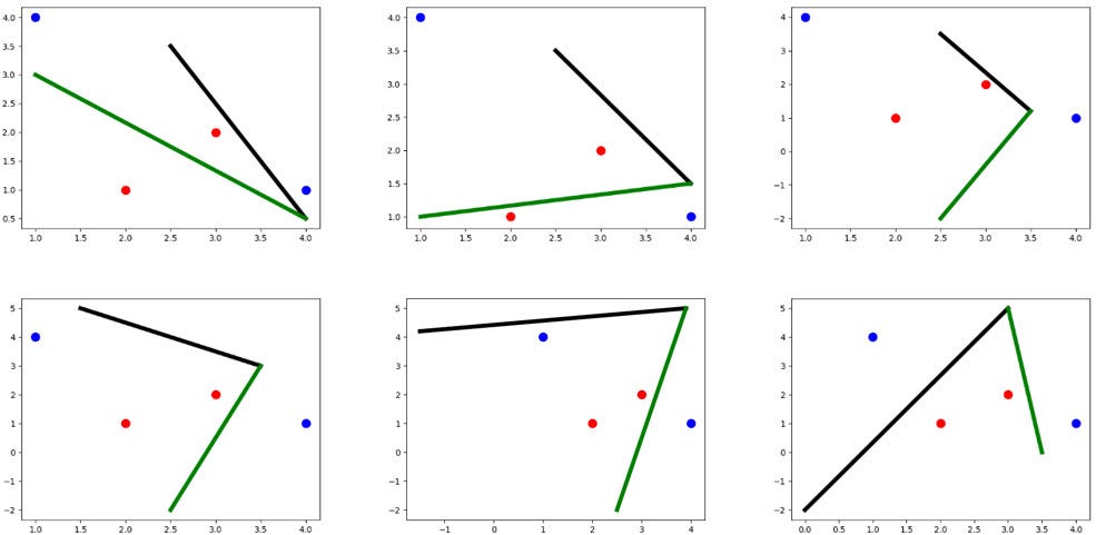
In this example, there is overlap between the 2 classes. Thus, we cannot use just a single line to split the data. We can easily deduce that the minimum number of lines is 2. One of their arrangements is given below. Note that this is not the only way of classifying the data correctly.
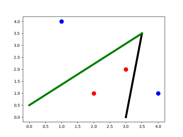
After knowing that the number of required lines is 2, then the network will have 2 hidden neurons in the first hidden layer, where each neuron produces a line.
The next question is, “How many hidden layers are required?” Remember that one hidden layer creates the lines using its hidden neurons. The proceeding hidden layer connects these lines. The number of connections defines the number of hidden neurons in the next hidden layer.
Based on this explanation, we have to use 2 hidden layers, where the first layer has 2 neurons and the second layer has 1 neuron. Because there are just 2 lines, then there will be just a single connection (i.e. just single hidden neuron in the second hidden layer). We can use the output neuron to connect the lines created by the neurons of the first hidden layer. Thus, we avoided creating a second hidden layer.
Note that reducing the number of hidden layers and neurons helps to increase the speed of the learning process. Finally, the conclusion is to use 1 hidden layer with 2 hidden neurons.
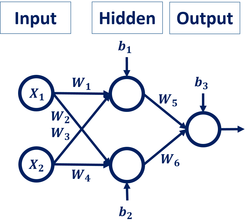
Here’s the ANN architecture. The network has 6 weights and 3 bias values for a total of 9 parameters to be optimized. Note that there’s a difference between parameter and hyperparameter. There are techniques for selecting the best values for the parameter, but not so much for hyperparameters.
When training the ANN, the parameter values are updated according to an optimizer, such gradient descent. Each time the parameters changes, the lines are rearranged. For example, the following figure shows a sample evolution of the lines from an initial state (top-left) to the point where we’re separating the classes correctly (bottom-right).
Python Implementation
After deciding the best number of hidden layers and neurons, the next step is to implement the ANN in Python. The scikit-learn Python library is used for that purpose.
Below is the Python code for creating an ANN using sklearn.neural_network.MLPClassifier(). This function has an argument named hidden_layer_sizes, which accepts a tuple defining the number of neurons per each layer. It’s set to (2,) to reflect that there is just a single hidden layer with 2 hidden neurons. All other arguments are set to their default values except for the max_iter, which is set to 1000.
This argument refers to the maximum number of iterations that the ANN goes through for training. Its default value is 200, according to its the documentation. It is set to a value higher (1,000) to ensure finding a better solution.
import sklearn.neural_network
import numpy
import matplotlib.pyplot

input_data = numpy.array([[1, 4],
                          [4, 1],
                          [3, 2],
                          [2, 1]])
output_data = numpy.array([0, 0, 1, 1])

my_neural_network = sklearn.neural_network.MLPClassifier(hidden_layer_sizes=(2,), max_iter=1000)

my_neural_network.fit(X=input_data, y=output_data)

labels = my_neural_network.predict(X=input_data)
print("Predicted Labels:", labels)
The network is trained using the fit() function, which accepts the training data inputs and their class labels. After being trained, the network predicts the class label of the training data. Here are the predicted class labels:
It’s obvious that the network made incorrect predictions. Does it mean that the selected number of hidden layers and hidden neurons is not optimal? The answer is NO.
In this tutorial, we want to highlight that there are many parameters and hyperparameters in machine learning models. Just selecting a bad value for one of them may affect the entire learning process and cause incorrect predictions.
In order to escape from this trouble, study each parameter/hyperparameter well in order to select its best value. After that, be sure that the incorrect result is caused by another parameter/hyperparameter. We studied the number of hidden layers and hidden neurons and concluded that 1 hidden layer with 2 hidden neurons is optimal. Thus, the incorrect results are, surely, caused by another parameter/hyperparameter.
In ANNs, the initial weights and bias values play a critical role in successful model training. In the previous example, the ANN is initialized by values that did not give the correct results. If we train the ANN another time, there will likely be new initial values that may enhance the prediction accuracy.
After re-training the ANN, the network successfully classified each sample correctly. The predicted labels are as follows:
We can print the weights and bias values of the trained ANN using the coef_ and intercepts_ properties as given below:
The values are as given below. The weights array has 2 sub-arrays. The first sub-array represents the weights between the input and the hidden layer. Its shape is 2×2 because there are 2 input neurons and 2 hidden neurons. The second sub-array has just 2 weights because it connects the hidden layer that has just 2 hidden neurons by the output layer neuron.
The bias array also has 2 sub-arrays. The first one represent the bias values for the 2 hidden neurons. The remaining sub-array has just one bias value for the output neuron.
When the prediction results are incorrect, it can be easy to follow an incorrect path for solving the issue. One way this can happen is by adding more hidden layers and neurons. The problem may be accidentally solved, and the predictions results end up being correct after adding more layers.
What may be happening in this situation is that the training process got repeated, and thus the weights and the bias values were re-initialized. The new initial values helped the model reach better prediction accuracy than before.
But the prediction accuracy isn’t actually enhanced due to the addition of new hidden layers or neurons. This is why you need to make sure that the selected value for a given hyperparameter is almost optimal.
In order to initialize the parameters to selected values, we can edit the coefs_ and intercepts_ properties of the trained NN.
After solving the first example, let’s discuss another example in which more hidden layers and neurons are used.
Example 2
The data used in the second example is given in the table below.
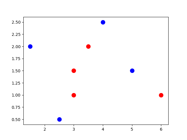
In order to decide the number of hidden layers and neurons, the graph of this data is given in the next figure.
After looking at the data, we can easily deduce that there’s a minimum of 4 lines required to separate the 2 classes. Here’s one arrangement of the lines.
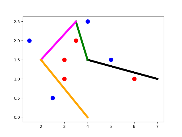
Because there are 4 lines required, there are 4 hidden neurons in the first hidden layer to produce them. Next, we need to again connect these lines together.
Because there’s more than one connection among the lines, we have to use other hidden layers. The second hidden layer connects the lines together to produce curves (i.e. each curve consists of 2 lines), the third hidden layer connects the produced curves to produce other complex curves (i.e. each curve has 4 lines), and so on.
In our example, we can use 2 other hidden layers. The first one produces curves of 2 lines. This layer produces 2 curves in order to connect. There will be just one connection required to connect these curves. The connection can be created by the third hidden layer, which will just have a single hidden neuron.
Remember that in binary classification problems there’s a neuron in the output layer that can create this connection. Thus, we can avoid using the third hidden layer and connect the curves produced by the second hidden layer using the output layer neuron.
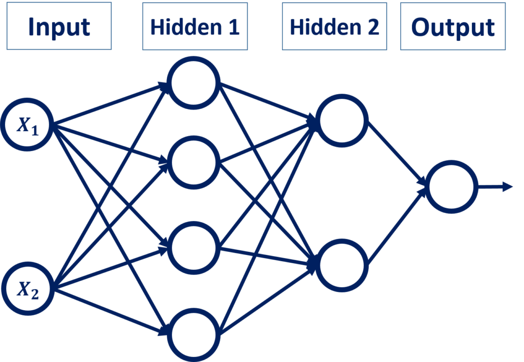
As a result, the ANN will have 2 hidden layers, where the first layer has 4 neurons and the second layer has 2 neurons.
The ANN architecture is given below. There’s a total of 18 weights and 7 bias values.
As we did before, we can start building the ANN using scikit-learn, according to the following code. Note that the accuracy will not be 100% from the first trial due to the reasons we previously discussed.
import sklearn.neural_network
import numpy
import matplotlib.pyplot

input_data = numpy.array([[5, 1.5],
                          [4, 2.5],
                          [1.5, 2],
                          [2.5, 0.5],
                          [6, 1],
                          [3.5, 2],
                          [3, 1.5],
                          [3, 1]])
output_data = numpy.array([0, 0, 0, 0, 1, 1, 1, 1])

my_neural_network = sklearn.neural_network.MLPClassifier(hidden_layer_sizes=(4,2), max_iter=1000)

my_neural_network.fit(X=input_data, y=output_data)
print("Weights:", my_neural_network.coefs_)
print("Bias:", my_neural_network.intercepts_)

labels = my_neural_network.predict(X=input_data)
print("Predicted Labels:", labels)
One version of the correct weights and bias values is given below:
Conclusion
This tutorial practically answers a frequently asked question about artificial neural networks, which is “what is the best architecture to use?”. By creating a 2D graph of the data, it’s very easy to decide how many hidden layers to use and also how many hidden neurons to use for each layer.
The strategy is to investigate the graph and place lines that separate the classes correctly (given a classification problem). Every line corresponds to a hidden neuron. Each connection between 2 lines represents a hidden neuron is a successive hidden layer.
By deciding the best number of hidden neurons and hidden layers, you reduce the effort of successfully building an ANN that fits your data.
For Contacting the Author
- E-mail: [email protected]
- LinkedIn: https://linkedin.com/in/ahmedfgad
- KDnuggets: https://kdnuggets.com/author/ahmed-gad
- TowardsDataScience: https://towardsdatascience.com/@ahmedfgad
- GitHub: https://github.com/ahmedfgad
Comments 0 Responses