Overcoming overfitting in image classification using data augmentation

Imagine you have trained an image classification model whose performance seems a bit poor—did you know there’s more you can do to improve such a model and reduce its bias? You’ve done a lot in creating your model pipeline and then building a predictive model using neural networks, yet its not improving as you expected

In these cases, as a first step I’d recommend you try implementing data augmentation.

In this tutorial, we’ll be looking at what data augmentation is all about and how we can apply this technique in improving the performance of our ML models, and image classification models specifically.

Data augmentation is a strategy that enables practitioners to significantly increase the diversity of data available for training models, without actually collecting new data. We can say data augmentation is a strategy focused on regeneration of more images from already-available ones. And more specifically, it’s a technique that helps us to reproduce an image in another form or dimension.

The image below gives us an idea of what we are about to do. This is an image of a dog but appears like the image was taken several times from various direction; but the truth is, this image was augmented to generate others. What this technique helps us to do to our algorithm performance includes:

Reduction in model bias towards a particular class of data to other classes. That is, it helps the algorithm generalize well.
Increases number of samples in less represented class present in the data (by augmenting original samples into creating more samples).

Introduction

To get started, I’ll be using an existing dataset many of us are likely already familiar with—the cat and dog dataset from Kaggle. Before we can augment this dataset, however, we first need to build a data pipeline. Once we complete these first steps, we’ll dive into data augmentation.

Building your data pipeline

For every problem you’re trying to solve with ML, you need to create a series of processes your data need to go through before modeling. This pipeline could and often does include the following:

Resizing dimensions of the input image
Conversion of images into arrays
Image filtering (not compulsory)
Image scaling (up scaling or down scaling)

For the sake of this tutorial, we’ll focus on 1 and 2, just to help get you started.

Instead of using TensorFlow Data (tf.data) to load our data, we’ll do this manually so that we can better understand the basics of how to load image data into an array. The code below helps us achieve this:

train_dir = '/root/.kaggle/training_set/training_set'
test_dir = '/root/.kaggle/test_set/test_set'
default_dir = '/root/.kaggle'

train_cat, train_dog, test_cat, test_dog = [], [],[],[]
def get_data():
    os.chdir(default_dir)
    # get data's on training cat
    current_dir = train_dir+'/cats'
    os.chdir(current_dir)
    train_data_cat = os.listdir()
    train_cat.extend(train_data_cat)
    
    # get data's on training dog
    current_dir = train_dir +'/dogs'
    os.chdir(current_dir)
    train_data_dog = os.listdir()
    train_dog.extend(train_data_dog)
    
    # get data's on test cat
    current_dir = test_dir+'/cats'
    os.chdir(current_dir)
    test_data_cat = os.listdir()
    test_cat.extend(test_data_cat)
    
    # get data's on test dog
    current_dir = test_dir +'/dogs'
    os.chdir(current_dir)
    test_data_dog = os.listdir()
    os.chdir(default_dir)
    test_dog.extend(test_data_dog)
    return

get_data()

We can basically check the amount of data that needs to be loaded using the code below:

print('Number of cats in our train data is: ', len(train_cat))
print('Number of dog in our train data is: ', len(train_dog))
print('Number of cats in our test data is: ', len(test_cat))
print('Number of dogs in our test data is: ', len(test_dog))
print('Total training data is: ', len(train_cat)+len(train_dog))
print('Total test data is: ', len(test_cat)+len(test_dog))

Now let’s look at how to manually load our data using the image class in Keras. We load in the data as a non-gray scale image of dimension 224 by 224. We do this by setting gray_scale to False:

import numpy as np
np.random.seed(100)

import keras
from keras.preprocessing import image

train_images = []
train_target = []
test_images = []
test_target = []


for i in train_cat:
    try:
        directory = train_dir + '/cats/' + i
        img = image.load_img(directory, target_size = (224,224), grayscale = False)
        img=image.img_to_array(img)
        img = img/255
        train_images.append(img)
        os.chdir(default_dir)
        train_target.append(0)
    except OSError as err:
        continue

for i in train_dog:
    try:
        directory = train_dir + '/dogs/' + i
        img = image.load_img(directory, target_size = (224,224), grayscale = False)
        img=image.img_to_array(img)
        img = img/255
        train_images.append(img)
        os.chdir(default_dir)
        train_target.append(1)
    
    except OSError as err:
        continue
    
    
for i in test_cat:
    try:
        directory = test_dir + '/cats/' + i
        img = image.load_img(directory, target_size = (224,224), grayscale = False)
        img=image.img_to_array(img)
        img = img/255
        test_images.append(img)
        os.chdir(default_dir)
        test_target.append(0)
    except OSError as err:
        continue

for i in test_dog:
    try:
        directory = test_dir + '/dogs/' + i
        img = image.load_img(directory, target_size = (224,224), grayscale = False)
        img=image.img_to_array(img)
        img = img/255
        test_images.append(img)
        os.chdir(default_dir)
        test_target.append(1)
    
    except OSError as err:
        pass

You can convert the manually-appended images as a list of arrays into arrays by the doing the following :

train_images = np.array(train_images)
test_images = np.array(test_images)
train_target = np.array(train_target)
test_target = np.array(test_target)
train_images.shape, test_images.shape, train_target.shape, test_target.shape

Now that we have all images read as an array, let’s move on to building our model.

Building our model

We’ll be building a custom model with the following things in mind:

An input network that takes in images of dimension 224 by 224 by 3, with a ReLU activation function.
An initial 2-dimensional convolution layer with 32 filters, where each filter size is 7 by 7.
A 2-dimensional max pooling layer for the first convolution layer with kernel size of 2 by 2.
A second 2-dimensional convolution layer with 16 filters, where each filter size is 5 by 5 with a ReLU activation function.
A 2-dimensional max pooling layer for the second convolution layer, with kernel size of 2 by 2.
A third 2-dimensional convolution layer with 8 filters, where each filter size is 5 by 5 with a ReLU activation function.
A 2-dimensional max pooling layer for the third convolution layer with kernel size of 2 by 2.
A flattened layer (to pass in all information into a fully connected layer).
An hidden layer of 300 neurons with a ReLU activation function.
An hidden layer of 100 neurons with a ReLU activation function.
An output layer of 2, since we want the model to predict the probability that an input image belongs to either class Dog or class Cat.

To write all of this in TensorFlow, we have:

model = models.Sequential()
model.add(layers.Conv2D(32, (7,7), activation='relu', input_shape=(224,224, 3)))
model.add(layers.MaxPooling2D((2, 2)))
model.add(layers.Conv2D(16, (5, 5), activation='relu'))
model.add(layers.MaxPooling2D((2, 2)))
model.add(layers.Conv2D(8, (2, 2), activation='relu'))
model.add(layers.MaxPooling2D((2, 2)))
model.add(layers.Flatten())
model.add(layers.Dense(300, activation='relu'))
model.add(layers.Dense(100, activation='relu'))
model.add(layers.Dense(2, activation = 'softmax'))
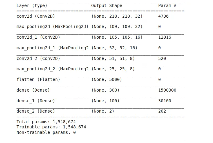
model.summary()

And we have this as the model summary. This network isn’t computationally intensive, as you can see—it’s trained on just 1.5 million params to give a unique result, compared to models with 300 million params.

So far so good — you’ve done a solid job designing your network from the above code. Now that you’re done with this, let’s compile the network we just built and then feed in the data fit needs to learn from. The code below helps us solve this.

We compile the network by running, model.compile and then passing in the necessary arguments. Finally, to make the model begin its learning process we use the fit attribute of the model and then pass in the data for it to learn from. This model will be trained for 10 epochs only— you can select whatever number you desire, but be careful, you don’t want your model to run forever.

We’ve chosen an Adam optimizer and categorical cross-entropy as our loss function. Finally, our target metric will be accuracy.

model.compile(optimizer='adam',
              loss=tf.keras.losses.SparseCategoricalCrossentropy(from_logits=True),
              metrics=['accuracy'])

history = model.fit(train_images, train_target, epochs=10, 
                    validation_data=(test_images, test_target))

If we look at the results of our model training above, we can see that the model began learning while training at 50% till it almost reached 100%, but on the validation data, it kicked off from 50% and began to maintain its pace at about 68%.

As such, the graph below makes us to understand that, when the model was learning from the training data, it learned all patterns and information; this is why it was almost a 100 percent accurate when evaluated.

But when we fed it validation data it hadn’t seen before, and we compared the result with the actual result; it was about 68% accurate in predicting the image classes correctly. We can basically say it has learned the training data too well and performed worse than expected on an unseen data.

68% is OK, but not so good when compared to the rate at which it was learning from its training data, which is 97%. This is a sign of overfitting. This brings us to some outlined solutions below:

Data augmentation
Regularization techniques (like dropouts)

Data augmentation explained

Data augmentation is a collection of techniques applied to image processing. In the real world, this collection of techniques is used alongside data pipelines to improve model performance by reducing data bias and improve model generalization.

When we talk about model performance for image classification, we mean this—The performance of a model in all its predicted classes is determined by the performance of the model on the least represented class. With data augmentation, we can basically solve this by regenerating more samples for the under-represented class(es) in order to have equal representation of all classes to be predicted. This diversity in data helps the model generalize, while also reducing bias.

Here’s how it works. With data augmentation, we can generate more data from the existing data we already have. All you need to do is make your model see the data it has been seeing in a new dimension. TensorFlow gives us the flexibility of doing this by using the image generator class present in its data pre-processing library.

This image generator gives us the flexibility of generating more images by executing any of the following techniques:

Image rotation
Zoom
Image flipping
Image scaling
Image cropping
Adding noise to your images

To augment your data, you have to first import the image data generator from Keras. Instantiate the classes for train and validation data separately. Then go specify the parameters you want to auto generate from existing data, like horizontal flip, rotation (by specifying the rotating angle), and others, as mentioned above:

from tensorflow.keras.models import Sequential
from tensorflow.keras.layers import Dense, Conv2D, Flatten, Dropout, MaxPooling2D
from tensorflow.keras.preprocessing.image import ImageDataGenerator

#initialize your train generator and validation generator
train_image_generator = ImageDataGenerator(rescale=1./255) # Generator for our training data
validation_image_generator = ImageDataGenerator(rescale=1./255) # Generator for our validation data

batch_size = 100
target_size = (224,224)
image_gen = ImageDataGenerator(rescale=1./255, horizontal_flip=True)
train_data_gen = image_gen.flow_from_directory(batch_size=batch_size,
                                               directory=train_dir,
                                               shuffle=True,
                                               target_size=target_size)
val_data_gen = validation_image_generator.flow_from_directory(batch_size=batch_size,
                                                              directory=test_dir,
                                                              target_size=target_size,
                                                              class_mode='binary')

Implementing data augmentation

Image flipping

To flip your images, try the following code below by setting horizontal_flip to True. This will select random images from your train data and flip to create new, augmented data:

image_gen = ImageDataGenerator(rescale=1./255, horizontal_flip=True)
train_data_gen = image_gen.flow_from_directory(batch_size=batch_size,
                                               directory=train_dir,
                                               shuffle=True,
                                               target_size=target_size)

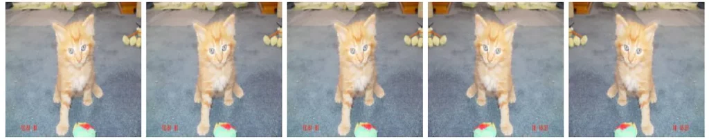
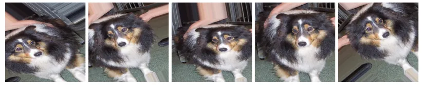
Image rotation

To rotate an image, try the following code below by experimenting with the rotation angle—here, I’ll set mine to 45 degrees. And I have the following code below:

image_gen = ImageDataGenerator(rescale=1./255, rotation_range=45)

train_data_gen = image_gen.flow_from_directory(batch_size=batch_size,
                                               directory=train_dir,
                                               shuffle=True,
                                               target_size=target_size)

augmented_images = [train_data_gen[0][0][0] for i in range(5)]

Image zoom

To zoom in on an image, this zoom range is specified to be between 0–1. As such, setting your zoom range to 0.7 means your zoom will vary randomly between 0 and 70%. So to do this, you need to specify the image zoom range. For this case, we’ll set it to 0.6 (that is, 60% of the maximum zoom):

# zoom_range from 0 - 1 where 1 = 100%.
image_gen = ImageDataGenerator(rescale=1./255, zoom_range=0.5) # 

train_data_gen = image_gen.flow_from_directory(batch_size=batch_size,
                                               directory=train_dir,
                                               shuffle=True,
                                               target_size=target_size)

augmented_images = [train_data_gen[0][0][0] for i in range(5)]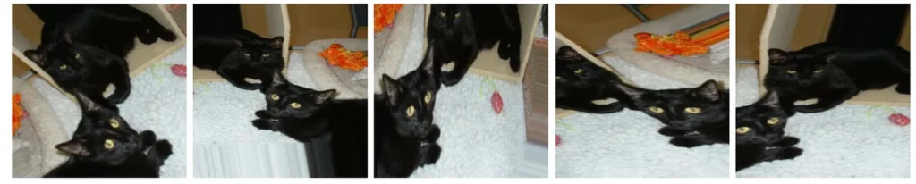

Now let’s put all of this together and evaluate the same model to see if these data augmentation techniques helped improve its performance:

image_gen_train = ImageDataGenerator(
                    rescale=1./255,
                    rotation_range=45,
                    width_shift_range=.15,
                    height_shift_range=.15,
                    horizontal_flip=True,
                    zoom_range=0.5
                    )

train_data_gen = image_gen_train.flow_from_directory(batch_size=batch_size,
                                                     directory=train_dir,
                                                     shuffle=True,
                                                     target_size=target_size,
                                                     class_mode='binary')


image_gen_val = ImageDataGenerator(rescale=1./255)v

val_data_gen = image_gen_val.flow_from_directory(batch_size=batch_size,
                                                 directory=test_dir,
                                                 target_size=target_size,
                                                 class_mode='binary')

#using the same model
model = models.Sequential()
model.add(layers.Conv2D(32, (7,7), activation='relu', input_shape=(224,224, 3)))
model.add(layers.MaxPooling2D((2, 2)))
model.add(layers.Conv2D(16, (5, 5), activation='relu'))
model.add(layers.MaxPooling2D((2, 2)))
model.add(layers.Conv2D(8, (2, 2), activation='relu'))
model.add(layers.MaxPooling2D((2, 2)))
model.add(layers.Flatten())
model.add(layers.Dense(300, activation='relu'))
model.add(layers.Dense(100, activation='relu'))
model.add(layers.Dense(2, activation = 'softmax'))
model.summary()

# complie the model
model.compile(optimizer='adam',
              loss=tf.keras.losses.SparseCategoricalCrossentropy(from_logits=True),
              metrics=['accuracy'])

# train the generator
epochs = 10
history = model.fit_generator(
    train_data_gen,
    steps_per_epoch=8005// batch_size,
    epochs=epochs,
    validation_data=val_data_gen,
    validation_steps=2023// batch_size
)

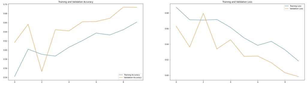
Below is a comparative look at model performance—we can see that there’s been some improvement in our model. While training, the model was accurately able to predict 69% of the data, and while validating it on unseen data, it was able to predict 66%of the data accurately.

So what has data augmentation done for us has helped in making this model generalize by reducing the rate at which it assumes the majority of the data to be of a particular class.

This is good in the sense that, if our model is able to learn accurately 80–90% of this same data, we can be more than sure that this same model won’t perform less than this range in real-world conditions.

However, this still isn’t good enough. The performance range of the model while training on unseen data is between 65–70%; we desire something as close as 95–100%. One of the things we can do is to increase the number of training epochs, or better still add some more regularization techniques—but we won’t cover that here, maybe in my next post.

Conclusion/model comparison

If you look at the model result, without augmentation and with augmentation, you will discover that there’s a significant reduction in model over fitting. Our model was able to generalize.

This helps validate that data augmentation helps to reduce over fitting and aids in model generalization. One more thing you can do to improve the model performance is to improve your model architecture.

The model architecture built in this tutorial has 3 convolutional layers of 32, 16, and 8 filters respectively; and a fully connected layer of 2 hidden layers (300 neurons in the first hidden layer and 100 neurons in the second hidden layer).

This architecture was selected to show that computational neural architectures can struggle to generalize; simple computation could get the job done just as well, which would be less cost-intensive compared to huge neural architectures that require more compute power.

I hope you learned a lot. To learn more about data augmentation, check out the official TensorFlow tutorial here: