Image Compression Using Different Machine Learning Techniques

In this post, we’re going to investigate the field of image compression and it’s applications in real world. We’ll explore various machine and deep learning techniques for image compression and inspect their pros and cons, and their practical feasibility in real-world scenarios.

So let’s get started!

What is image compression?

Image compression refer to reducing the dimensions, pixels, or color components of an image so as to reduce the cost of storing or performing operations on them. Some image compression techniques also identify the most significant components of an image and discard the rest, resulting in data compression as well.

Image compression can therefore be defined as a data compression approach that reduces the data bits needed to encode an image while preserving image details.

Why are image compression techniques needed?

Listed below are some of the potential applications of image compression:

1. Data takes up lesser storage when compressed. As a result, this allows more data to be stored with less disk space. This is especially useful in healthcare, where medical images need to be archived, and dataset volume is massive.
2. Some image compression techniques involving extracting the most useful components of the image (PCA), which can be used for feature summarization or extraction and data analysis.
3. Federal government or security agencies need to maintain records of people in a pre-determined, standard, and uniform manners. Thus, images from all sources need to be compressed to be of one uniform shape, size, and resolution.

Types of image compression

Types of image compression can be categorized by their ability to re-create the original image from its compressed form.

Lossy Compression

Lossy compression, as its name suggests, is a form of data compression that retains useful image details while discarding a few bits in order to reduce its size or to extract important components. Thus, in lossy compression, data is irreversibly lost and the original image cannot be completely re-created.

Lossless Compression

Lossless compression is a form of data or image compression under which any sort of data loss is avoided, and thus, compressed images are larger in size. However, the original image can be re-constructed using this kind of image compression.

Let’s take a closer look at how we can use machine learning techniques for image compression.

Image Compression using principal component analysis

Principal component analysis(PCA) is a technique for feature extraction — so it combines our input variables in a specific way, at which point we can drop the least important variables while still retaining the most valuable parts of all of the variables. PCA results in the development of new features that are independent of one another.

Briefly listing the steps of PCA below:

1. Scale the data by subtracting the mean and dividing by std. deviation.
2. Compute the covariance matrix.
3. Compute eigenvectors and the corresponding eigenvalues.
4. Sort the eigenvectors by decreasing eigenvalues and choose k eigenvectors with the largest eigenvalues, with these becoming the principal components.
5. Derive the new axes by re-orientation of data points according to the principal components.

To learn more about PCA, please refer to this article.

Image compression using PCA

The principal components, when sorted in the order of their eigenvalues, preserve most of the information in the dataset within the first principal component, the rest in the second, and so on.

Thus, we can preserve most of the details in an image by applying PCA. We can detect the number of principal components required to preserve variance by a certain percentage—say, 95% or 98%—and then apply PCA to transform the data space.

All the steps mentioned above will be followed in the same manner, and in the end we can create the compressed image by using this transformed data space.

It’s very space-efficient, since an image with n*m pixels or dimensions (say 28*28=784) can be preserved by a very small number of principal components (just around 20–30).

Source to get started:

Image compression using k-means clustering

K-means clustering is a prototype-based, partitional clustering technique that attempts to find a user-specified number of clusters (k), which are represented by their centroids.

Briefly listing the steps of k-means clustering below:

1. We first choose k initial centroids, where k is a user-specified parameter; namely, the number of clusters desired.
2. Each point is then assigned to the closest centroid, and each collection of points assigned to a centroid is called a cluster.
3. The centroid of each cluster is then updated based on the points assigned to the cluster.
4. We repeat the assignment and update steps until no point changes clusters, or similarly, until the centroids remain the same.

To learn more about k-means clustering, please refer to this article.

Image compression using k-means clustering

As discussed earlier in this post, image compression, in some techniques, involves reducing the color components of the image. With k-means clustering, this is what we’re doing.

We pre-define the value of k as the number of color components that we want to preserve in the image. The rest of the k-means algorithm is performed according to the above-mentioned steps.

With an increase in the value of k, as the number of clusters increases, the image will get closer and closer to the original image, but at the cost of more disk space for storage and a higher computational cost. We can experiment with the values of k to get desirable results.

We can also calculate the within-cluster sum of squared error to gain insight on whether the clusters are well fitted and correctly assigned or not, since it provides us with the variance of the cluster centroids.

Source to get started:

Image compression using GANs

In generative adversarial networks, two networks train and compete against each other, resulting in mutual improvisation. The generator misleads the discriminator by creating compelling fake inputs and tries to fool the discriminator into thinking of these as real inputs . The discriminator tells if an input is real or fake.

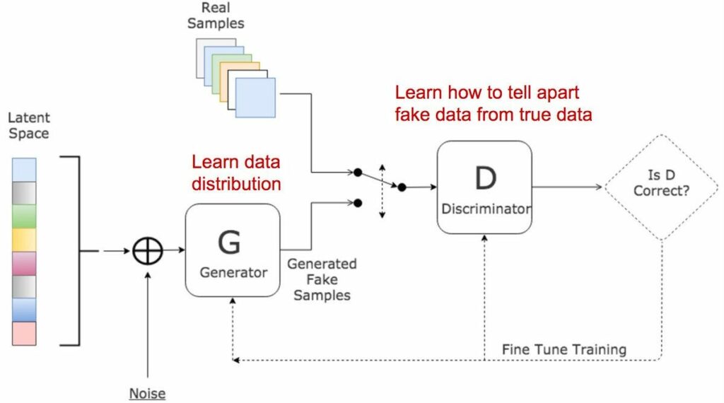
There are 3 major steps in the training of a GAN:

1. Using the generator to create fake inputs based on random noise, or in our case, random normal noise.
2. Training the discriminator with both real and fake inputs (either simultaneously by concatenating real and fake inputs, or one after the other, the latter being preferred).
3. Train the whole model: the model is built with the discriminator combined with the generator.

To learn more about GANs, please refer to this article.

Conditional GANs (CGAN)

Conditional GANs are slightly different from traditional GANs. In a conventional GAN, the output images have no bound; that is, there is no way to determine what the generator would produce.

But in conditional GANs, along with the images as input, additional information is provided as input to the generator and discriminator so that the produced output would be in accordance with the additional information.

For example, while generating new handwritten digits with a GAN, a network that’s trained on the MNIST dataset will produce random digits—there’s no way to track its output or predict which digit the generator produces next.

However, in CGANs, we can provide the image and the class label (one hot encoded vector informing which digit the image corresponds to) as an input to the generator as well as the discriminator. Thus, our model would be conditioned on class labels. Therefore, this additional information helps the generator produce digits.

We start with the assumption that s(additional information) is given and that we want to use the GAN to model the conditional distribution Px|s. In this case, both the generator G(z,s) and discriminator D(z,s) have access to the side information s, leading to the divergence

Image compression using GANs

The CGAN is used similarly to an encoder-decoder model, such that the encoder encrypts the information in the image in a latent map by compressing the image and limiting the number of color components, and then this map is used by the decoder (generator) to develop a compressed image according to the information provided.

With the help of an encoder E and a quantized value q, we encode the image i to get a compressed representation of the image as w = q(E(i)). The decoder/generator G then tries to generate an image i= G(z) that’s consistent with the image distribution Px and also resembles the original image to a certain degree.

Source to get started:

Here is a detailed and thorough research paper that discusses using CGAN for the task of image compression. It’s well written and I highly recommend you to give it a try to gain better insights on generative compression.

Conclusion

In this post, we addressed the real-world problem of image compression. Compressed images enhance the efficiency of data storage and transfer. Additionally, we discussed how we can apply various machine learning algorithms and deep neural nets to perform the task with ease.

This post contains references to my previous posts on PCA, k-means clustering and GANs. I recommend reading those as well to get a better understanding of their applications here.

All feedback is welcome and appreciated—I’d love to hear what you think of this article.