
Deploying memory-hungry deep learning algorithms is a challenge for anyone who wants to create a scalable service. Cloud services are expensive in the long run.
Deploying models offline on edge devices is cheaper, and has other benefits as well. The only disadvantage is that they have a paucity of memory and compute power.
This blog explores a few techniques that can be used to fit neural networks in memory-constrained settings.
Different techniques are used for the “training” and “inference” stages, and hence they are discussed separately.
Training
Certain applications require online learning. That is, the model improves based on feedback or additional data.
Deploying such applications on the edge places a tangible resource constraint on your model. Here are 4 ways you can reduce the memory consumption of such models.
1. Gradient Checkpointing
Frameworks such as TensorFlow consume a lot of memory for training. During a forward pass, the value at every node in the graph is evaluated and saved in memory. This is required for calculating the gradient during backprop.
Normally this is okay, but when models get deeper and more complex, the memory consumption increases drastically. A neat sidestep solution to this is to recompute the values of the node when needed, instead of saving them to memory.

However, as shown above, the computational cost increases significantly. A good trade-off is to save only some nodes in memory while recomputing the others when needed.
These saved nodes are called checkpoints. This drastically reduces deep neural network memory consumption. This is illustrated below:

2. Trade speed for memory (Recomputation)
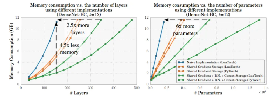
Extending on the above idea, we can recompute certain operations to save time. A good example for this is the Memory Efficient DenseNet implementation.
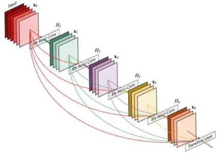
DenseNets are very parameter efficient, but are also memory inefficient. The paradox arises because of the nature of the concatenation and batchnorm operations.
To make convolution efficient on the GPU, the values must be placed contiguously. Hence, after concatenation, cudNN arranges the values contiguously on the GPU. This involves a lot of redundant memory allocation.
Similarly, batchnorm involves excess memory allocation, as explained in this paper. Both operations contribute to a quadratic growth in memory. DenseNets have have a large number of concatenations and batchnorms, and hence they are memory inefficient.
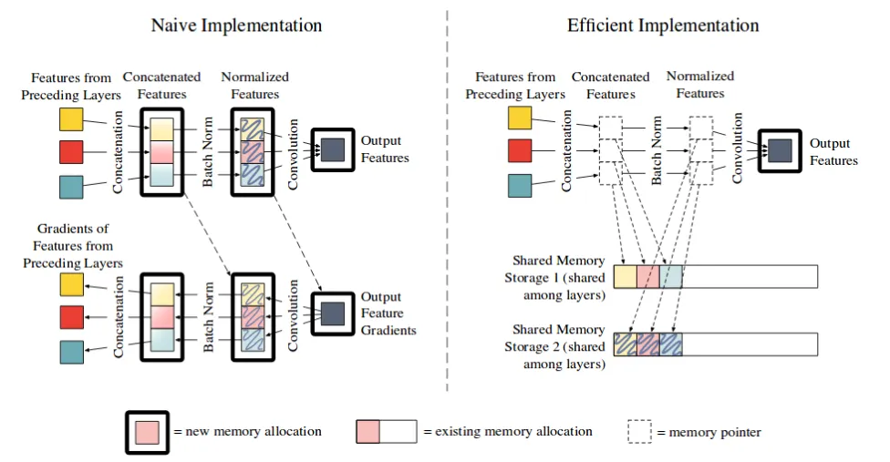
A neat solution to the above involves two key observations.
Firstly, concatenation and batchnorm operations are not time intensive. Hence, we can just recompute the values when needed, instead of storing all the redundant memory.
Secondly, instead of allocating “new” memory space for the output, we can use a “shared memory space” to dump the output.
We can overwrite this shared space to store output of other concatenation operations. We can recompute the concatenation operation for gradient calculation when needed.
Similarly, we can extend this for the batchnorm operation. This simple trick saves a lot of GPU memory, in exchange for slightly increased compute time.
3. Reduce Precision
In an excellent blog, Pete Warden explains how neural networks can be trained with 8-bit float values. There are a number of issues that accrue because of reduction in precision, some of which are listed below:
- As stated in this paper, “activations, gradients, and parameters” have very different ranges. A fixed-point representation would not be ideal. The paper a claims that a “dynamic fixed point” representation would be an excellent fit for low precision neural networks.
- As stated in Pete Warden’s other blog, lower precision implies a greater deviation from the exact value. Normally, if the errors are totally random, they have a good chance of canceling each other out. However, zeros are used extensively for padding, dropout, and ReLU. An exact representation of zero in the lower precision float format may not be possible, and hence might introduce an overall bias in the performance.
4. Architecture Engineering for Neural Networks
Architecture engineering involves designing the neural network structure that best optimizes accuracy, memory, and speed. There are several ways by which convolutions can be optimized space-wise and time-wise.
- Factorize NxN convolutions into a combinations of Nx1 and 1xN convolutions. This conserves a lot of space while also boosting computational speed. This and several other optimization tricks were used in newer versions of the Inception network. For a more detailed discussion, check out this blog post.
- Use Depthwise Separable convolutions as in MobileNet and Xception Net. For an elaborate discussion on the types of convolutions, check out this blog post.
- Use 1×1 convolutions as a bottleneck to reduce the number of incoming channels. This technique is used in several popular neural networks.
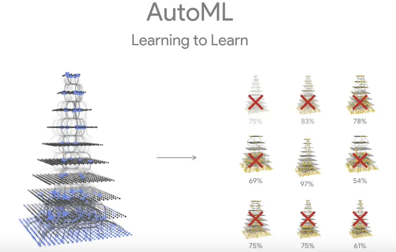
An interesting solution is to let the machine decide the best architecture for a particular problem. Neural Architecture Search uses machine learning to find the best neural network architecture for a given classification problem.
When used on ImageNet, the network formed as a result (NASNet) was among the best performing models created so far. Google’s AutoML works on the same principle.
Inference
Fitting models for edge inference is relatively easier. This section covers techniques that can be used to optimize your neural network for such edge devices.
1. Removing “Bloatware”
Machine learning frameworks such as TensorFlow consume a lot of memory space for creating graphs. This additional space is useful for speeding up the training processes, but it isn’t used for inference.
Hence, the part of the graph used exclusively for training can be pruned off. Let’s call this part of the graph bloatware.
For TensorFlow, it’s recommended to convert model checkpoints to frozen inference graphs. This process automatically removes the memory-hungry bloatware.
Graphs from model checkpoints that throw Resource Exhausted Error can sometimes be fit into memory when converted to a frozen inference graph.
2. Pruning Features
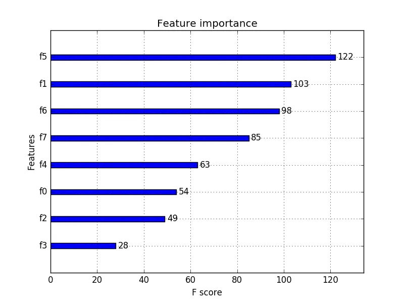
Some machine learning models on Scikit-Learn (such as Random Forest and XGBoost) output an attribute named feature_importances_.
This attribute represents the significance of each feature for the classification or regression task. We can simply prune the features with the least significance. This can be extremely useful if your model has an excessively large number of features that you cannot reduce by any other method.
Similarly, in neural networks, a lot of weight values are close to zero. We can simply prune those connections. However, removing individual connections between layers creates sparse matrices.
There is work being done on creating efficient inference engines (hardware), which can handle sparse operations seamlessly.
However, most machine learning frameworks convert sparse matrices to their dense form before sending them to the GPU.
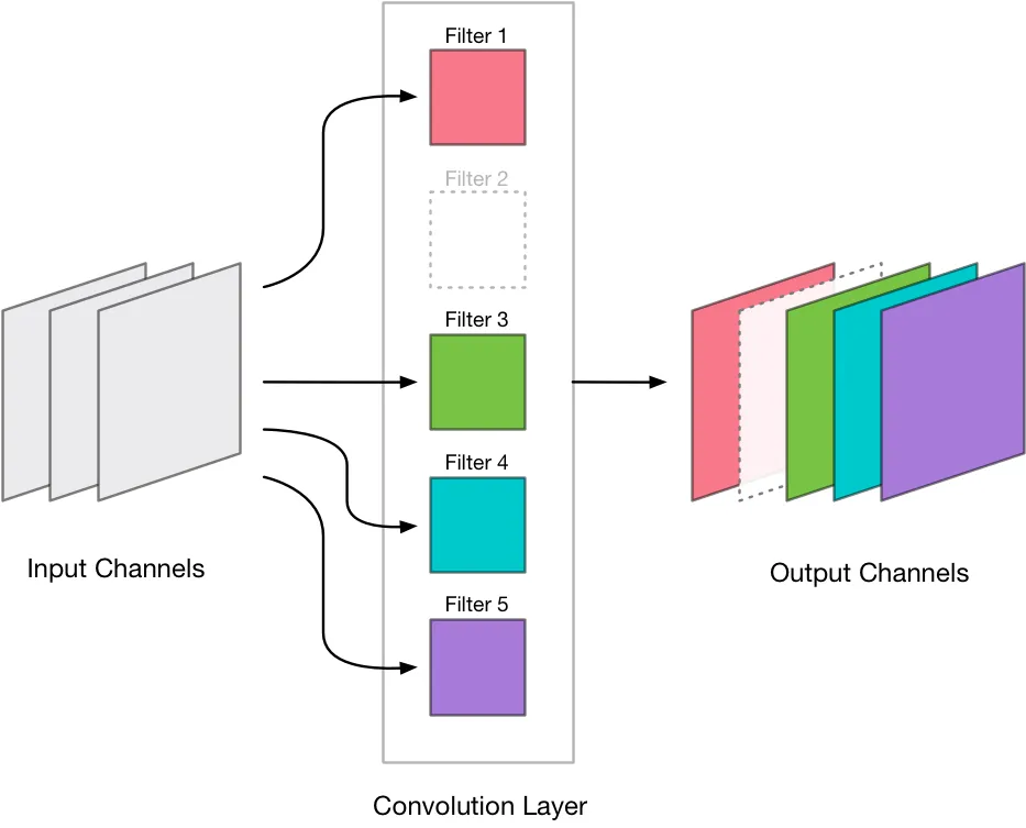
Instead, we can remove insignificant neurons and slightly retrain the model. For CNNs, we can remove entire filters, too. Research and experiments have shown that we could retain most of the accuracy, while obtaining a massive reduction in size, by using this method.
3. Weight Sharing
To best illustrate weight sharing, consider the example given in this Deep Compression paper. Consider a 4×4 weight matrix. It has 16 32-bit float values. We require 512 bits (16 * 32) to represent the matrix.
Let us quantize the weight values to 4 levels, but let’s preserve their 32-bit nature. Now, the 4×4 weight matrix has only 4 unique values.
The 4 unique values are stored in a separate (shared) memory space. We can give each of the 4 unique values a 2-bit address (Possible address values being 0, 1, 2, and 3).
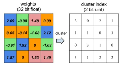
We can reference the weight values by using the 2-bit addresses. Hence, we obtain a new 4×4 matrix with 2-bit addresses, with each location in the matrix referring to a location in the shared memory space. This method requires 160 bits (16 * 2 + 4 * 32) for the entire representation. We obtain a size reduction factor of 3.2.
Needless to say, this reduction in size comes with an increase in time complexity. However, the time to access shared memory would not be a severe time penalty.
4. Quantization and Lower Precision (Inference)
Recall that we covered reduction in precision in the training part of this blog. For inference, reduction in precision is not as cumbersome as for training.
The weights can just be converted to a lower precision format and be shipped off to inference. However, a sharp decrease in precision might require a slight readjustment of weight values.
5. Encoding
The pruned and quantized weights can be size-optimized further by using encoding. Huffman encoding can represent the most frequent weight values with a lower number of bits. Hence, at the bit level, a Huffman encoded string takes a smaller space than a normal string.
Deep compression explores encoding using lossless compression techniques such as Huffman. However, research has explored the use of lossy compression techniques as well. The downside to either method is the overhead of translation.
6. Inference Optimizers
We’ve discussed some great ideas so far, but implementing them from scratch would take quite some time. This is where inference optimizers kick in. For instance, Nvidia’s TensorRT incorporates all of these great ideas (and more) and provides an optimized inference engine given a trained neural network.
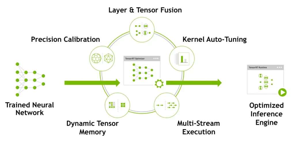
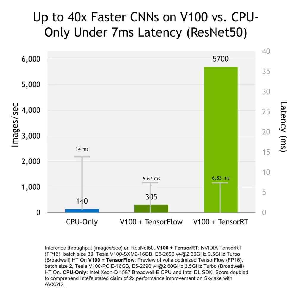
Moreover, TensorRT can optimize the model such that it can make better use of Nvidia’s hardware. Below is an example where a model optimized with TensorRT uses Nvidia’s V100 more efficiently.
7. Knowledge Distillation
Instead of performing fancy optimization techniques, we can teach smaller models to mimic the performance of beefy, larger models. This technique is called knowledge distillation, and it’s an integral part of Google’s Learn2Compress.
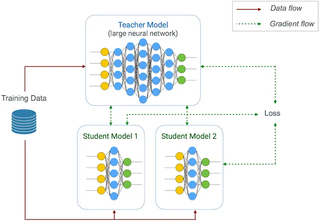
By using this method, we can force smaller models that can fit on edge devices to reach the performance levels of larger models. The drop in accuracy is reported to be minimal. You can refer to Hinton’s paper on the same for more information.
Discuss this post on Reddit and Hacker News.
Comments 0 Responses