In the first part of this series, I introduced deep learning in JavaScript—we explored why you should consider using Javascript for deep learning, and then went on to create a neural network to predict areas acutely affected by forest fires.
As you might have noticed, if you read part one or are otherwise familiar with TF.js, both training and inference happened directly in the browser. While training in the browser can be fast and effective for small datasets, it quickly becomes intractable as the data scales. This is mostly because the amount of storage assigned to a browser is minimal.

In order to leverage the power of deep learning, especially for perceptual tasks like image recognition, object detection, or pose estimation, you’ll need access to more compute power.
To solve this challenge, we need to perform training at the backend (server-side). But instead of using Python, we can leverage the TensorFlow.js node version (tfjs-node).
This TensorFlow.js (node) version can be installed in a node environment and, according to the creators, has access to a low-level C++ runtime, the same runtime used by Python TensorFlow.
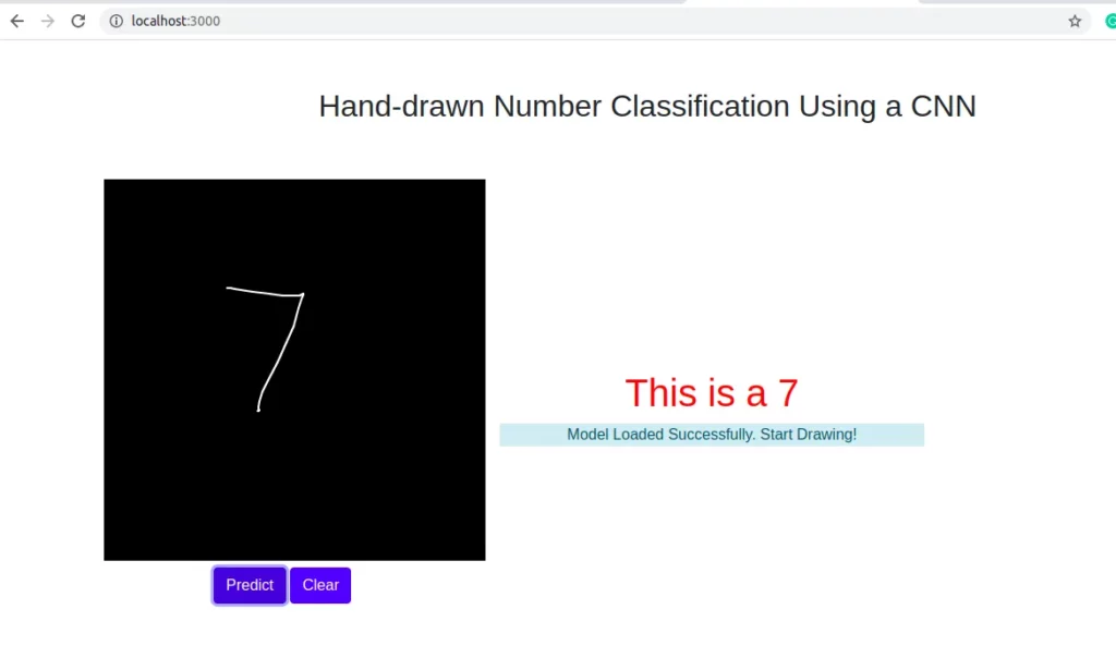
In this article, we’re going to create an application that can recognize hand-drawn digits in the browser. Below is the end product of what we’ll create:

Link to full code
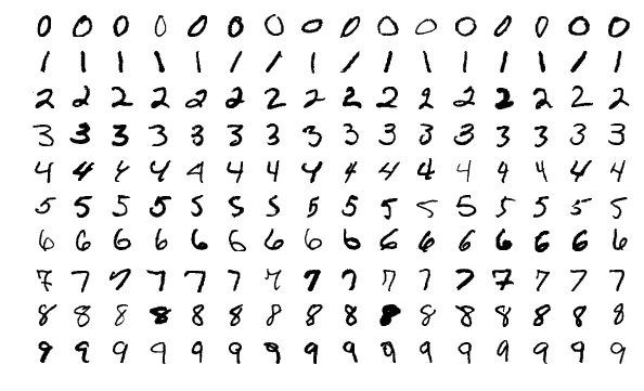
In order to create this demo, we need to download the MNIST handwritten digits datasets. You can download it from Kaggle here.

The dataset contains 42,000 grayscale images that have been converted into pixel values and stored in a CSV format. Each row of the dataset contains 745 columns, with the first column as the label, and each pixel value has a range of [0–255]. We’re going to create a convolutional neural network (CNN) to help us classify these digits, which run from 0–9.
Before we move on, I’ll assume you’re familiar with CNNs in general and understand some of the basic concepts around convolution, dropout, and so on. If you don’t understand these concepts, I’ll advise you to take a bit of time to familiarize yourself with them before proceeding to the next sections. You can find good tutorials on the subject here:
Now let’s get started!
Setting up your workspace
First, you need to have Node.js installed on your computer. If you don’t, you can find installation details on the official website here.
Next, open a terminal in your project directory and install express-generator.
express-generator will help us quickly create a simple scaffold Node app. We’ll build on top of this so that we don’t bother ourselves with directory structures.
To use express-generator, run the following command in your terminal
You can configure the express-generator by setting the view engine with the — view command. Although we won’t be rendering views in this application, I prefer to use handlebars as my default.
The directory structure generated by express-generator is shown below:
├── app.js
├── bin
│ └── www
├── package.json
├── public
│ ├── images
│ ├── javascripts
│ └── stylesheets
├── routes
│ ├── index.js
│ └── users.js
└── views
Our application is going to be composed of two parts. The backend for training, and the frontend for inference. The app.js file and other scripts (model.js and data.js) which we’ll create shortly will handle all data ingestion and model training, while the files inside the public folder will handle the UI and model inference.
Now go ahead and create the two extra scripts (model.js and data.js) and a dataset folder (dataset) in the root directory. Your directory structure should now look like this:
├── dataset
├── app.js
├── bin
│ └── www
├── data.js
├── model.js
├── package.json
├── public
│ ├── images
│ ├── javascripts
│ └── stylesheets
├── routes
│ ├── index.js
│ └── users.js
└── views
Before we continue, go ahead and download the train dataset from Kaggle and move it to the dataset folder.
├── dataset
│ ├── train.csv
Next, let’s add the TensorFlow.js package to our app. Open the package.json file and add the @tensorflow/tfjs-node and argparse dependencies, as shown below:
{
  "name": "mnist-classification",
  "version": "0.0.0",
  "private": true,
  "scripts": {
    "start": "node ./bin/www"
  },
  "dependencies": {
    "@tensorflow/tfjs-node": "1.7.4",
    "argparse": "*",
    "cookie-parser": "~1.4.4",
    "debug": "~2.6.9",
    "express": "~4.16.1",
    "http-errors": "~1.6.3",
    "morgan": "~1.9.1"
  }
}
The argparse package will help us parse command-line arguments used for model training customization, which we’ll see shortly.
Next, let’s look at the model training scripts and understand their respective functions.
The main entry point of our application (app.js)
The app.js file is the entry point of our app at the backend. It receives and parses training arguments like the number of epochs, model saving path, etc., and calls the corresponding functions to start model training.
const express = require('express');
const path = require('path');
const cookieParser = require('cookie-parser');
const logger = require('morgan');
const argparse = require('argparse');

const model = require('./model')


const indexRouter = require('./routes/index');

const app = express();

app.use(logger('dev'));
app.use(express.json());
app.use(express.urlencoded({ extended: false }));
app.use(cookieParser());
app.use(express.static(path.join(__dirname, 'public')));


const parser = new argparse.ArgumentParser({
    description: 'TensorFlow.js-Node MNIST Classification.',
    addHelp: true
});
parser.addArgument('--epochs', {
    type: 'int',
    defaultValue: 5,
    help: 'Number of epochs to train the model for.'
});
parser.addArgument('--batch_size', {
    type: 'int',
    defaultValue: 128,
    help: 'Batch size to be used during model training.'
})
parser.addArgument('--model_save_path', {
    type: 'string',
    help: 'Path to which the model will be saved after training.'
});
parser.addArgument('--train_mode', {
    type: 'int',
    help: 'Train with full dataset ot not on node backend (1=true, 0=false).'
});

const args = parser.parseArgs();


if (args.train_mode == 1) {
    console.log("Loading Full Dataset. Sit back and relax")
    model.trainModel(args)
}

if (args.train_mode == 0) {
    console.log("Loading Train and Test Dataset. Sit back and relax")
    model.trainModel(args)
}


module.exports = app;- The first set six lines of code basically require all the packages we’ll be using. They’re automatically added by express-generator. The next line requires the model package, which we’ll see shortly.
- The lines of code before the argparse section are all generated by express and are mostly used for view rendering and parsing request objects.
- The next part is the parser arguments. Here we use the argparse library to require some arguments from the command line. Specifically, you can specify the epoch size ( — epochs) and batch size ( — batch_size), specify whether to train the model without splitting into train and test sets or not ( — train_mode), and finally specify a local file path to save the trained model to ( — model_save_path).
Ingesting data and pre-processing it (data.js)
The data.js file handles everything involved with data ingestion and preparation. Here we’ll leverage tf.data.csv in TensorFlow to read in our data. Copy and paste the code below:
const tf = require('@tensorflow/tfjs-node');


const BASE_PATH = "file:///home/dsn/personal/Tfjs/TensorFlowjs_Projects/mnist-classification/dataset/";
const TRAIN_DATA = `${BASE_PATH}train.csv`;
const IMAGE_WIDTH = 28
const IMAGE_HEIGHT = 28
const IMAGE_CHANNEL = 1
const NUM_CLASSES = 10;
const DATA_SIZE = 42000
const NUM_TRAIN_DATA = 38000
const NUM_TEST_DATA = DATA_SIZE - NUM_TRAIN_DATA

const TENSOR_DATA = []
const LABEL = []


async function loadData() {
    const csvDataset = tf.data.csv(TRAIN_DATA, {
        columnConfigs: {
            label: { isLabel: true }
        }
    });
    await csvDataset.forEachAsync(row => process(row));

}


async function process(row) {
    TENSOR_DATA.push(Object.values(row['xs']))
    LABEL.push(Object.values(row['ys'])[0])
}


exports.MnistClass = class MnistDataset {
    constructor() {
        this.Xtrain = null
        this.Xval = null
        this.ytrain = null
        this.ytest = null
    }

    async startDataLoading(train_mode) {
        // dat = new MnistDataset()
        await loadData()
        if (train_mode == 0) {
            //partial training
            this.Xtrain = tf.tensor(TENSOR_DATA.slice(0, NUM_TRAIN_DATA)).reshape([NUM_TRAIN_DATA, IMAGE_HEIGHT, IMAGE_WIDTH, IMAGE_CHANNEL]).div(255.0)
            this.Xtest = tf.tensor(TENSOR_DATA.slice(NUM_TRAIN_DATA)).reshape([NUM_TEST_DATA, IMAGE_HEIGHT, IMAGE_WIDTH, IMAGE_CHANNEL]).div(255.0)
            this.ytrain = tf.oneHot(tf.tensor1d(LABEL.slice(0, NUM_TRAIN_DATA), 'int32'), NUM_CLASSES);
            this.ytest = tf.oneHot(tf.tensor1d(LABEL.slice(NUM_TRAIN_DATA), 'int32'), NUM_CLASSES);
        } else {
            //full training
            this.Xtrain = tf.tensor(TENSOR_DATA).reshape([DATA_SIZE, IMAGE_HEIGHT, IMAGE_WIDTH, IMAGE_CHANNEL]).div(255.0)
            this.ytrain = tf.oneHot(tf.tensor1d(LABEL, 'int32'), NUM_CLASSES);

        }

    }

}- First (and importantly), we require the TensorFlow package. We’ll use this to read and process the CSV dataset.
- Next, we set the full file path of the dataset file. The full file path (including the “file://” prefix) is important; otherwise, TensorFlow will throw an error when reading the file.
- Next, we set some important parameters for our dataset. The MNIST dataset contains 28 x 28 grayscale images. This means that if we’re to perform convolution on each using a CNN, we would have to reshape each image to 28 x 28 x 1, corresponding to height x width x channel.
- Next, we set the number of classes we are predicting (10), the total training dataset size, and the held-out test size.
- Next, we create two empty arrays to hold our processed data and labels.
- In the next code block, we load the CSV dataset by passing the data path to the tf.data.csv function. We specify the target of the dataset as the column (label), and this instructs TensorFlow to extract the target into a separate array. Then, we call a processing function for each row in the CSV file.
- The processing function simply extracts the features called xs in TensorFlow.js, and the target (ys). It then pushes them to the arrays we initialized earlier.
- Next, we wrap the dataset functionality into a class. This provides a clean API for loading and retrieving the dataset. In the loadData function of the Mnistclass we created, we perform some important pre-processing:
Creating and training the model (model.js)
The model.js file houses our CNN. Here we create the model, perform training and evaluation, and then save it to a specified folder. Let’s walk through the code below:
const tf = require('@tensorflow/tfjs-node');
const data = require('./data')

const IMAGE_WIDTH = 28
const IMAGE_HEIGHT = 28
const IMAGE_CHANNEL = 1


function getModel() {

    const model = tf.sequential();
    model.add(tf.layers.conv2d({
        inputShape: [IMAGE_HEIGHT, IMAGE_WIDTH, IMAGE_CHANNEL],
        filters: 32,
        kernelSize: 3,
        activation: 'relu',
    }));
    model.add(tf.layers.conv2d({
        filters: 32,
        kernelSize: 3,
        activation: 'relu',
    }));
    model.add(tf.layers.maxPooling2d({ poolSize: [2, 2] }));
    model.add(tf.layers.conv2d({
        filters: 64,
        kernelSize: 3,
        activation: 'relu',
    }));
    model.add(tf.layers.conv2d({
        filters: 64,
        kernelSize: 3,
        activation: 'relu',
    }));
    model.add(tf.layers.maxPooling2d({ poolSize: [2, 2] }));
    model.add(tf.layers.flatten());
    model.add(tf.layers.dropout({ rate: 0.25 }));
    model.add(tf.layers.dense({ units: 512, activation: 'relu' }));
    model.add(tf.layers.dense({ units: 10, activation: 'softmax' }));

    const optimizer = 'rmsprop';
    model.compile({
        optimizer: optimizer,
        loss: 'categoricalCrossentropy',
        metrics: ['accuracy'],
    });

    return model

}


exports.trainModel = async (args) => {
    const cnn_model = getModel()
    const train_mode = args.train_mode
    mnist = data.MnistClass
    dataset = new mnist()

    if (train_mode == 0) {
        //partial training with train and test set
        dataset.startDataLoading(train_mode).then(async () => {
            console.log("Data Loaded Successfully. Training started.")
            await cnn_model.fit(dataset.Xtrain, dataset.ytrain, {
                epochs: args.epochs,
                batchSize: args.batch_size,
                validationSplit: 0.2,
                callbacks: {
                    onEpochEnd: async (epoch, logs) => {
                        console.log(`EPOCH (${epoch + 1}): Train Accuracy: ${(logs.acc * 100).toFixed(2)}, Val Accuracy:  ${(logs.val_acc * 100).toFixed(2)}n`);
                    }
                }
            })

            console.log("Testing on Final Test Set")
            const eval = cnn_model.evaluate(dataset.Xtest, dataset.ytest)
            console.log(`Test Loss: ${(eval[0].dataSync()[0]).toFixed(3)}, Test Accuracy:  ${(eval[1].dataSync()[0] * 100).toFixed(2)}n`);

        })

    } else {
        //full mode training
        dataset.startDataLoading(train_mode).then(async () => {
            console.log("Full Data Loaded Successfully. Training started.")
            await cnn_model.fit(dataset.Xtrain, dataset.ytrain, {
                epochs: args.epochs,
                batchSize: args.batch_size,
                callbacks: {
                    onEpochEnd: async (epoch, logs) => {
                        console.log(`EPOCH (${epoch + 1}): Train Accuracy: ${(logs.acc * 100).toFixed(2)}n`);
                    }
                }
            })

            console.log('*************************n')
            console.log(`Saving Model to ${args.model_save_path}`)
            await cnn_model.save(args.model_save_path)
            console.log(`Saved model to path: ${args.model_save_path}n`);
        })

    }

}- First, we import the TensorFlow package, as this will help us create the CNN model. Then we require the data module, which will be used to feed data to our model.
- Next, we create a function getModel. This function helps us create the CNN. The CNN is structured to have 2 conv layer and a maxpool layer immediately following it. After the conv-maxpool pair, we add a flatten layer. Then we specify the filter size and individual kernel sizes.
- After the flatten layer, we add a dropout layer to help to curb overfitting, then passed the result to a dense layer with 512 neurons. And finally, we add our output layer and used a softmax activation function.
- Next, we compile the model by specifying the optimizer to use (rmsprop), the loss function—categorical cross-entropy since we’re predicting more than 2 classes—and finally accuracy as our metric.
- In the final function (trainModel), we first initialize the MNIST dataset class we created earlier, then load the data and their corresponding labels.
- Next, we confirm if the training mode is set to full or not. In partial training mode (0), we split the dataset into distinct train and test sets and calculate an evaluation metric. This helps us fine-tune the network. In full mode (1), we use the entire dataset to train the CNN and then save it to the specified folder.
Partial Model training (train_mode=0)
The partial training mode function contains the following:
- The fit method, which takes parameters like the epochs and batch size parsed from the command line arguments and performs model training. Notice the ValidationSplit parameter? It informs TensorFlow of the percentage of data from the train set to set aside for validation. Here, we specify 20% of the data.
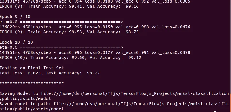
- Next, we added a callback that prints the accuracy on both the train and validation set at the end of every epoch during partial training.
- Next, we evaluate the model after training is complete. The evaluation is done on the held-out test set the model hasn’t seen before (validation). We also print the result to the console.
Full Model training (train_mode=1)
In the full training mode, we perform training on all available datasets, print the training logs at the end of every epoch, and finally, save the trained model to the specified folder. We’ll use this saved model for inference in the frontend of our application.
In your terminal opened in the root directory of your application, enter the following commands to start the partial training:
node app.js --train_mode=0 --epochs=10 --batch_size=64 --model_save_path='file:///home/personal/TensorFlowjs_Projects/mnist-classification/public/assets/model'
Experiment with different numbers for the epoch and batch size to see which gives higher accuracy. When you’re satisfied with the accuracy, you can move on to full model training mode.
Before you start full training, you first have to create a new folder in the public directory called assets. In the assets folder, create another folder called model. We’ll save our trained model file here. This also ensures we have access to the model files in the front end.
├── public
│ ├── assets
│ │ └── model
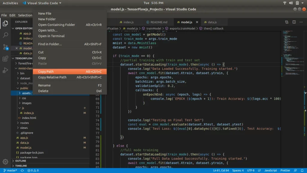
Next, obtain the full path to the model folder. In most OS’s, you can get this by right-clicking on the folder and copying the path link.
If you’re using VSCode like me, you can get the full path by right-clicking on the model folder and clicking Copy Path.

Next, in your terminal, set the train_mode to 1 and specify the model path you’ve copied, as shown below:
node app.js --train_mode=1 --epochs=10 --batch_size=64 --model_save_path='file:///home/personal/TensorFlowjs_Projects/mnist-classification/public/assets/model'
Now sit back, relax, and watch your model train.

When it’s all done training, the model will be saved to the specified path. You should see a model.json file and a weights.bin file.

Congratulations! You’ve just trained a convolutional neural network on a large dataset of handwritten images using TensorFlow.js in a Node environment.
In the next post, I’ll show you how to connect the frontend of this application and leverage the saved model for real-time and quick inference. As an extra feature, we’ll create an input canvas where we can draw a number and predict its class with TensorFlow.js.
If you have any questions, suggestions, or feedback, don’t hesitate to use the comment section below. Stay safe for now, and keep learning!

Connect with me on Twitter.
Connect with me on LinkedIn.

Comments 0 Responses