
Detecting objects, classifying them, and then keeping track of them is the biggest advancement in the deep learning area. There are many use cases of object detection in our day-to-day life; some examples are judging human behavior, activity trackers, some use in public sectors, crime detection, and many more.
In this article, I will help you deploy your own custom object detection based recommendation system to the web. In the end, you can interact with your real-time object detection and recommendation model using your web interface. Finally, you can host it over the cloud to access it everywhere, even with your mobile devices.
Software requirements
We will need a few libraries to run our model. We will be using Python 3 in our project. We will be deploying our object detection and recommender model using Flask. We will need OpenCV to process the image data. And, finally, we need TensorFlow to run our object detection model.
The data
The data I will be using in this article is of sunglasses. Our model will be trained on that sunglasses data. In the input, the user will be uploading his/her picture with sunglasses/eyeglasses. Our model will detect the glasses in the image and then the model will use the recommendation technique to display similar suggested images of sunglasses on the webpage.
Part 1: Creating a model for deployment
Our agenda here is to deploy our object detection based recommendation to the web. I will be focusing more on the deployment part but for your reference, I will first go through all the model development steps in brief.
Grab images for labeling
This is the first step. Here, you can go to Google and search for the pictures you want to build your custom system for or you can go around and take photos of objects and gather them for the model. This is your choice of how you want your model to be as batch images are faster but, if you take images by yourself, the images will be more realistic so accuracy can increase.
Label your images
Give a fair amount of time to this step as it is essential for your accuracy. You can use any tools for labeling your data. There is no automatic approach to label your custom data, you have to do it manually, and this is the most frustrating and time-consuming part of the object detention, but you will get a fruitful result if you give your dedication to this part. I have used the LabelImg tool for labeling. To know more about how the LabelImg tool works, please follow this article on how to label images for object detection.
Object detection model training
You must select the appropriate object detection algorithm. Here, we will be using the YOLO model. We will use Colab to train our model.
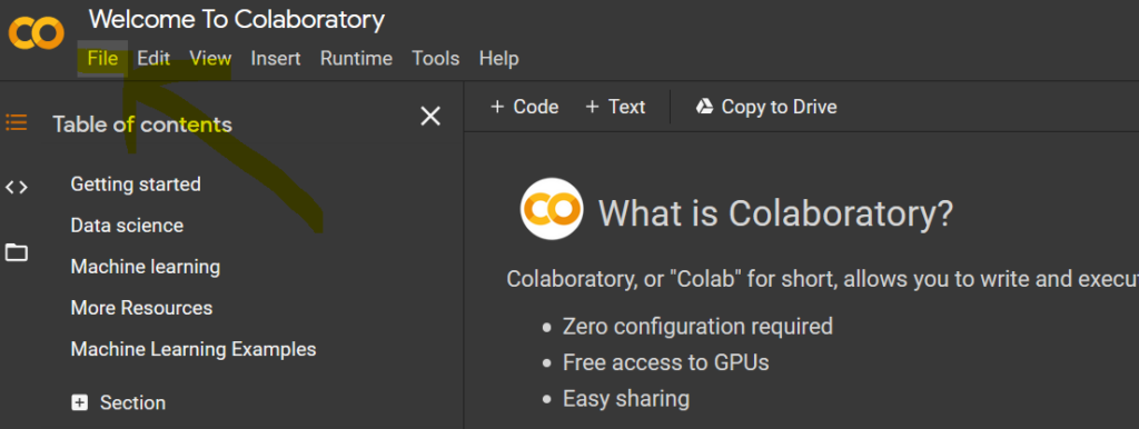
First, you need to launch the Jupyter notebook in Colab. You can do this by clicking on the file and selecting “New Notebook.”
Select runtime as “GPU” in the Runtime drop-down in the Colab.
Now we need to mount the drive with Colab. Use the code below in the notebook for mounting. One URL will generate—click on that to verify the mounting process.
from google.colab import drive
drive.mount('/content/gdrive')
!ln -s /content/gdrive/My Drive/ /mydrive
!ls /mydrive
We will then use the below code for the download darknet model for training our object detector. We need to enable GPU and CUDNN for faster model training and then make our (building) model suitable for GPU.
!git clone https://github.com/AlexeyAB/darknet
# verify CUDA
!/usr/local/cuda/bin/nvcc --version

# change makefile to have GPU and OPENCV enabled
%cd darknet
!sed -i 's/OPENCV=0/OPENCV=1/' Makefile
!sed -i 's/GPU=0/GPU=1/' Makefile
!sed -i 's/CUDNN=0/CUDNN=1/' Makefile
!sed -i 's/CUDNN_HALF=0/CUDNN_HALF=1/' Makefile
!make
Now, based on the number of classes, we need to make a change in the config file of the darknet model. Here we are using only a single class i.e. Glasses. The below code will help us make the required changes in the config file. Here, max_batches should be max (6000, no. of class * 2000) and the value of filters = (classes+5)*3, and the last thing we can find in the yolov4.cfg file is the “steps” where steps should be 80% and 90% of max batches.
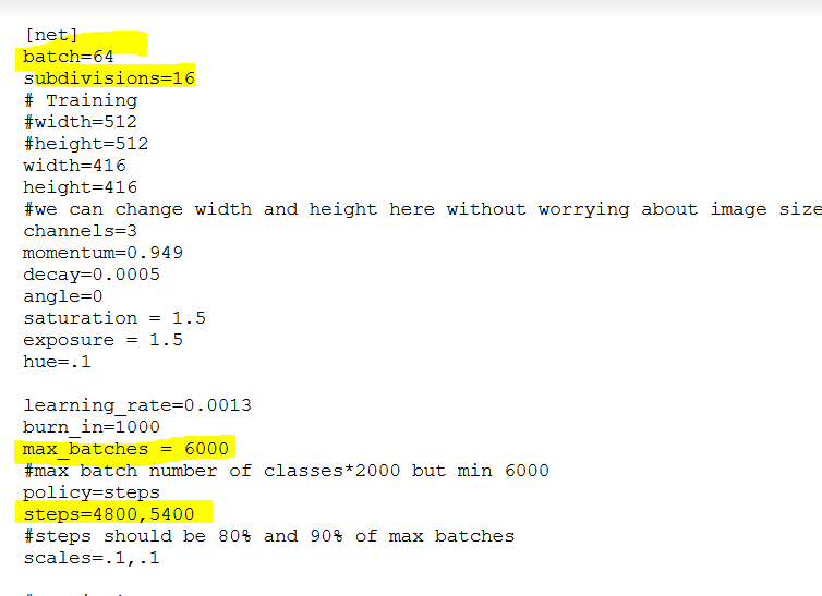
Type the below code in the next cell of the Jupyter notebook. It will make the necessary changes.
!sed -i 's/batch=1/batch=64/' cfg/yolov4.cfg
!sed -i 's/subdivisions=1/subdivisions=16/' cfg/yolov4.cfg
!sed -i 's/max_batches = 500500/max_batches = 6000/' cfg/yolov4.cfg
!sed -i '968 s@classes=80@classes=1@' cfg/yolov4.cfg
!sed -i '1056 s@classes=80@classes=1@' cfg/yolov4.cfg
!sed -i '1144 s@classes=80@classes=1@' cfg/yolov4.cfg
!sed -i '961 s@filters=255@filters=18@' cfg/yolov4.cfg        .
!sed -i '1049 s@filters=255@filters=18@' cfg/yolov4.cfg
!sed -i '1137 s@filters=255@filters=18@' cfg/yolov4.cfg
Now we need to define .names, .obj file, and the location where we need to save our model ( .weight file ).
!echo "Glasses" > data/obj.names
!echo -e 'classes= 1ntrain  = data/train.txtnvalid  = data/test.txtnnames = data/obj.namesnbackup = /mydrive/yolov4_v1' > data/obj.data
!mkdir data/obj
Download pre-trained weights.
!wget https://github.com/AlexeyAB/darknet/releases/download/darknet_yolo_v3_optimal/yolov4.weights
!wget https://github.com/AlexeyAB/darknet/releases/download/darknet_yolo_v3_optimal/yolov4.conv.137
Now we load the labeled data that we prepared earlier. We need to keep both the image and label file generated earlier within the same folder and zip it. After zipping, upload the folder to your Google Drive.
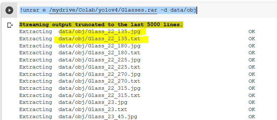
Use the below code for loading and arranging the data. I have kept the zipped file in “/mydrive/Colab/yolov4/Glasses.rar.” Accordingly, you can change the path as per your zipped file location.
!unrar e /mydrive/Colab/yolov4/Glasses.rar -d data/obj

import glob
import os
import re

txt_file_paths = glob.glob(r"data/obj/*.txt")
for i, file_path in enumerate(txt_file_paths):
    # get image size
    with open(file_path, "r") as f_o:
        lines = f_o.readlines()

        text_converted = []
        for line in lines:
            print(line)
            numbers = re.findall("[0-9.]+", line)
            print(numbers)
            if numbers:

                # Define coordinates
                text = "{} {} {} {} {}".format(0, numbers[1], numbers[2], numbers[3], numbers[4])
                text_converted.append(text)
                print(i, file_path)
                print(text)
        # Write file
        with open(file_path, 'w') as fp:
            for item in text_converted:
                fp.writelines("%sn" % item)
import glob
images_list = glob.glob("data/obj/*.jpg")
#Create training.txt file
file = open("data/train.txt", "w")
file.write("n".join(images_list))
file.close()
Finally, use the below command to start training your object detector. You will get a weight file in the same location you defined in the above step.
# Start the training
!./darknet detector train data/obj.data cfg/yolov4_training.cfg yolov4.conv.137 -dont_show
After getting your YOLO weight file from before, you need to convert the YOLO generated darknet model .weight file into TensorFlow serving so that we can serve it using TensorFlow to our webpage.
So, if you have reached here, cheers! You have done a great job. You are ready to move your model to production.
Darknet to TensorFlow Conversion
For darknet to TensorFlow conversion, you need to clone this directory https://github.com/pranjalAI/tensorflow-yolov4-tflite. You can clone it anywhere in your drive. After the clone, you need to enter in the cloned directory using a command prompt.
Installing Required Libraries
If you have Anaconda installed on your machine, then you need to follow the below steps to install all the required libraries in an environment. This will create a new environment. The environment name can be changed in the .yml file.
If you don’t have Anaconda installed, then follow the below steps using the pip command. However, I would suggest using Anaconda.
So, the new environment with respective dependencies has been created. Now, if you have used the Anaconda approach, then to use the newly created environment you need to activate it. And, if you are using pip, then you can skip this activation step.
Type the below command in your command prompt.
conda activate yolov4-gpu
Here “yolov4-gpu” is the environment name. You can change it in the .yml file.
Finally, you need to make two changes in your cloned folder that is “tensorflow-yolov4-tflite.”
First, copy and paste your custom .weights file which you used for your YOLO model training into the ‘data’ folder and copy and paste your custom .names into the ‘data/classes/’ folder.
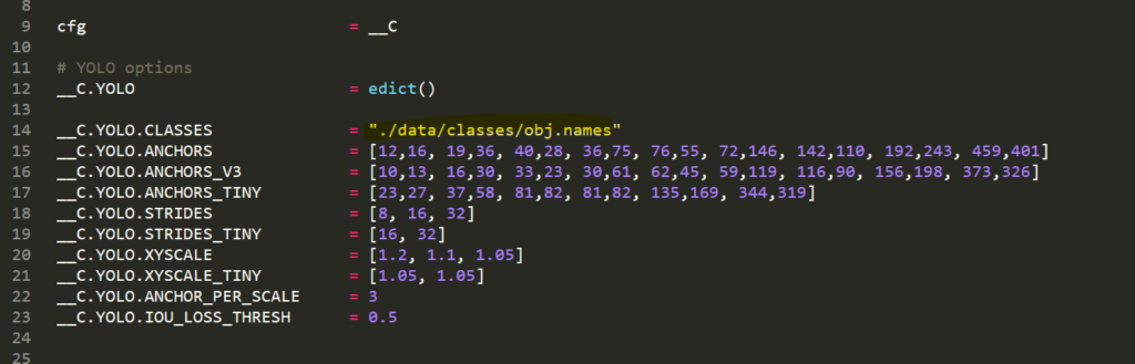
Second, on line 14 of ‘core/config.py’ file, update the code to point at your custom .names file as seen below. My custom .names file is called obj.names but yours might be named differently.
Here we go! Now, we need a single line of command to make the code TensorFlow compatible.
python save_model.py — weights ./data/your_weight_file.weights — output ./checkpoints/“check_point_name” — input_size 416 — model yolov4
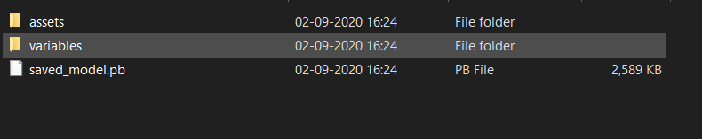
Here, 416 is the image size we have defined in our config file in the darknet config file. After running the above command you will get a .pb file, which we will use in our web app.
Part 2: Creating a web app with Flask
Using Flask to serve the TensorFlow model
We now have our TensorFlow served model .pb file ready. We need to serve it using Flask to our webpage. We will need a demo webpage to upload our image. I have that demo web page ready. You can get that repository from here.
After downloading the repository, you need to extract the data. There you will get a GlassDetectorAndRecommender.py file. This is your Flask file which will use the .pb file to perform the object detection on the web. We have used the histogram image matching technique in this Flask file to get the recommended similar images.
from __future__ import division, print_function
# coding=utf-8
import sys
import os
import glob
import re, glob, os,cv2
import numpy as np
import pandas as pd
import glass_detection
from shutil import copyfile
import shutil
from distutils.dir_util import copy_tree

# Flask utils
from flask import Flask, redirect, url_for, request, render_template
from werkzeug.utils import secure_filename
from gevent.pywsgi import WSGIServer

# Define a flask app
app = Flask(__name__)

for f in os.listdir("static\similar_images\"):
    os.remove("static\similar_images\"+f)

print('Model loaded. Check http://127.0.0.1:5000/')


@app.route('/', methods=['GET'])
def index():
    # Main page
    return render_template('index.html')


@app.route('/predict', methods=['GET', 'POST'])
def upload():
    if request.method == 'POST':
        # Get the file from post request
        f = request.files['file']

        # Save the file to ./uploads
        basepath = os.path.dirname(__file__)
        file_path = os.path.join(
            basepath, 'uploads', secure_filename(f.filename))
        f.save(file_path)

        # Make prediction
        similar_glass_details=glass_detection.getUrl(file_path)


        print("Checking for similar images.......")
        #getting similar images
        test_image = cv2.imread(file_path)
        gray_image = cv2.cvtColor(test_image, cv2.COLOR_BGR2GRAY)
        histogram_test = cv2.calcHist([gray_image], [0],
                                 None, [256], [0, 256])

        hist_dict={}
        for image in os.listdir("data\Data\"):
            try:
                img_to_compare = cv2.imread("data\Data\"+image)
                img_to_compare = cv2.cvtColor(img_to_compare, cv2.COLOR_BGR2GRAY)
                img_to_compare_hist = cv2.calcHist([img_to_compare], [0],
                                         None, [256], [0, 256])
                c=0
                i = 0
                while i
Congratulations on deploying your object detection based recommendation system on the web! We can now host it using any hosting service. Thanks for being here and keep enjoying data science.
Comments 0 Responses