Generative adversarial networks (GANs) are among the more significant advancements in deep learning in recent years. Previously, we used machine learning and deep learning techniques with a considerable amount of data to build a model to understand data by classifying them. But now, with GANs, we use an algorithm that generates data for us.
Two of the most commonly used and efficient generative models are Variational Autoencoders (VAE) and Generative Adversarial Networks (GAN).
A VAE learns a given distribution comparing its input to its output; this is good for learning hidden representations of data but is pretty bad for generating new data. This is mainly because we learn an averaged representation of the data; thus, the output becomes pretty blurry.
GANs, on the other hand, aims to generate data that looks like real data—this data can be image, text, audio, or video.
In this article, we’ll cover a detailed analysis of GANs, their implementation on mobile devices, and some of their limitations.
Generative Adversarial Networks (GANs): An overview
GANs consist of two different and separate neural networks. The first is the generator, and the second is the discriminator. The generator generates fake objects that look real, and the discriminator learns to distinguish real objects from fake/generated ones. The generator’s goal, then, is to trick the discriminator.
The game starts by collecting real objects. The generator cannot see real objects, but our discriminator is allowed to see them and is trained on them. The discriminator classifies target objects as real or fake and provides the probability that a given object is fake (i.e., has been generated).
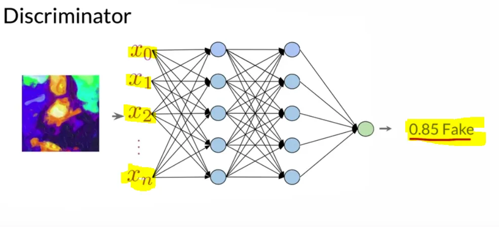
The discriminator is simply a neural network based on images (usually a CNN) that can classify objects as real or fake. It assigns the score to the generator’s fake object—and as soon as we observe that the generator generates good quality objects, and the probability of the discriminator classifying an image as the fake is below our threshold value, the game ends.
On the other hand, the generator uses a noise vector to generate random images. It takes the class (human face, dog, cat, document) and the noise vector as input and generates objects (image, video, music, or text) as output.
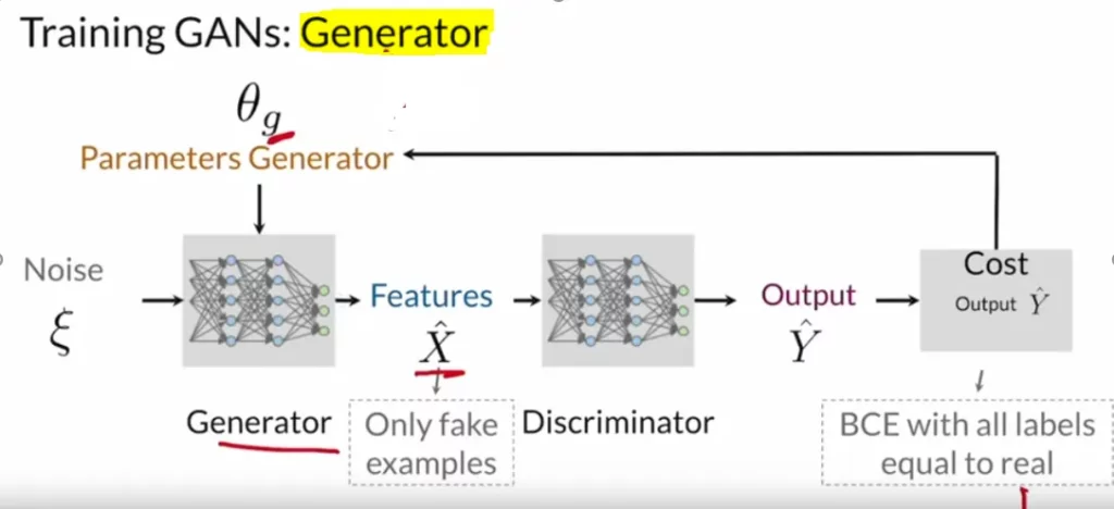
That generated object gets passed to the discriminator with the real one, without telling the discriminator which is real and which fake. And then the discriminator makes the prediction. Finally, the prediction gets compared with the desired label and calculates BCE loss. That loss helps the discriminator update its parameters.
At any given time, one model trains while others remain constant. If the discriminator’s weights get to update, the generator will be idle. And when the generator’s weights receive an update, the discriminator will remain constant.

In the end, our generator and the discriminator should be of a similar “skill level.” If the discriminator is superior, then the generator will not know in which direction to learn. Typically, you’ll need the generator to take multiple steps to improve itself for every step the discriminator takes.
Code Implementation
GANs have two separate neural networks. The first one is the Generator that generates the image and the second one is the discriminator that discriminates if the image is fake. The activation function for GANs is the Relu and for discriminator is Leaky Relu.
Generator’s Implementation
We start with the sequential layer then we add input layers with the shape of a random seed followed by the upsampling and convolutional layers. We can add several layers based on the model accuracy and the size of the memory we have. The more layers we will add, the complex our model will be; it will take more computation power. We use the Relu activation function for the overfitting issue and the batch normalization layers for the vanishing gradient problem, which happens due to complex models.
def build_generator(seed_size, channels):
    model = Sequential()

    model.add(Dense(4*4*256,activation="relu",input_dim=seed_size))
    model.add(Reshape((4,4,256)))

    model.add(UpSampling2D())
    model.add(Conv2D(256,kernel_size=3,padding="same"))
    model.add(BatchNormalization(momentum=0.8))
    model.add(Activation("relu"))

    model.add(UpSampling2D())
    model.add(Conv2D(256,kernel_size=3,padding="same"))
    model.add(BatchNormalization(momentum=0.8))
    model.add(Activation("relu"))

    # Output resolution, additional upsampling
    model.add(UpSampling2D())
    model.add(Conv2D(128,kernel_size=3,padding="same"))
    model.add(BatchNormalization(momentum=0.8))
    model.add(Activation("relu"))

    if GENERATE_RES>1:
      model.add(UpSampling2D(size=(GENERATE_RES,GENERATE_RES)))
      model.add(Conv2D(128,kernel_size=3,padding="same"))
      model.add(BatchNormalization(momentum=0.8))
      model.add(Activation("relu"))

    # Final CNN layer
    model.add(Conv2D(channels,kernel_size=3,padding="same"))
    model.add(Activation("tanh"))

    return model
Discriminator’s Implementation
We provide an image as input to our model, and then we add the convolutional layers followed by dropout. The dropout layer makes the model less complicated. Then we add the Leaky Relu as the activation function and batch normalization. And finally, we use the flatten layer and apply the sigmoid activation function with single output as a fake or not fake probability.
def build_discriminator(image_shape):
    model = Sequential()

    model.add(Conv2D(32, kernel_size=3, strides=2, input_shape=image_shape,
                     padding="same"))
    model.add(LeakyReLU(alpha=0.2))

    model.add(Dropout(0.25))
    model.add(Conv2D(64, kernel_size=3, strides=2, padding="same"))
    model.add(ZeroPadding2D(padding=((0,1),(0,1))))
    model.add(BatchNormalization(momentum=0.8))
    model.add(LeakyReLU(alpha=0.2))

    model.add(Dropout(0.25))
    model.add(Conv2D(128, kernel_size=3, strides=2, padding="same"))
    model.add(BatchNormalization(momentum=0.8))
    model.add(LeakyReLU(alpha=0.2))

    model.add(Dropout(0.25))
    model.add(Conv2D(256, kernel_size=3, strides=1, padding="same"))
    model.add(BatchNormalization(momentum=0.8))
    model.add(LeakyReLU(alpha=0.2))

    model.add(Dropout(0.25))
    model.add(Conv2D(512, kernel_size=3, strides=1, padding="same"))
    model.add(BatchNormalization(momentum=0.8))
    model.add(LeakyReLU(alpha=0.2))

    model.add(Dropout(0.25))
    model.add(Flatten())
    model.add(Dense(1, activation='sigmoid'))

    return model
Defining Loss & Optimizers
We need to define the loss functions for both generator and the discriminator. We will use the loss function as the binary cross-entropy loss because we have two classes fake and not fake. As our discriminator takes both the actual images and the real images, we use the combined loss. Finally, we use adam as an optimizer.
cross_entropy = tf.keras.losses.BinaryCrossentropy(from_logits=True)

def discriminator_loss(real_output, fake_output):
    real_loss = cross_entropy(tf.ones_like(real_output), real_output)
    fake_loss = cross_entropy(tf.zeros_like(fake_output), fake_output)
    total_loss = real_loss + fake_loss
    return total_loss

def generator_loss(fake_output):
    return cross_entropy(tf.ones_like(fake_output), fake_output)

generator_optimizer = tf.keras.optimizers.Adam(1.5e-4,0.5)
discriminator_optimizer = tf.keras.optimizers.Adam(1.5e-4,0.5)
Training our model
Out of the two models generator and the discriminator, we train one model at a time, and while switching to another model, we freeze the weights of another model. And, finally, when we start getting better accuracy, we can stop training the model and can use the generator model for our use. The discriminator model only helps us updating weights for our generator model.
@tf.function
def train_step(images):
  seed = tf.random.normal([BATCH_SIZE, SEED_SIZE])

  with tf.GradientTape() as gen_tape, tf.GradientTape() as disc_tape:
    generated_images = generator(seed, training=True)

    real_output = discriminator(images, training=True)
    fake_output = discriminator(generated_images, training=True)

    gen_loss = generator_loss(fake_output)
    disc_loss = discriminator_loss(real_output, fake_output)


    gradients_of_generator = gen_tape.gradient(
        gen_loss, generator.trainable_variables)
    gradients_of_discriminator = disc_tape.gradient(
        disc_loss, discriminator.trainable_variables)

    generator_optimizer.apply_gradients(zip(
        gradients_of_generator, generator.trainable_variables))
    discriminator_optimizer.apply_gradients(zip(
        gradients_of_discriminator,
        discriminator.trainable_variables))
  return gen_loss,disc_loss
Saving & Using Model for Mobile Devices
After training the model, we can save the file as a .pb format—a format compatible with some mobile platforms.
Then, we can simply:
- Create a new Android Studio app called GAN with all the defaults
- Add compile ‘org.tensorflow:tensorflow-android:+’ to the app’s build.gradle file
- Create a new assets folder and copy the GAN model files
- And a test blurry image there
We have two GANs models—the first one is for generating numbers, named gan_mnist.pb, and the second one is the pix2pix model that helps us enhance images.
Your project in Android Studio should now look like this:
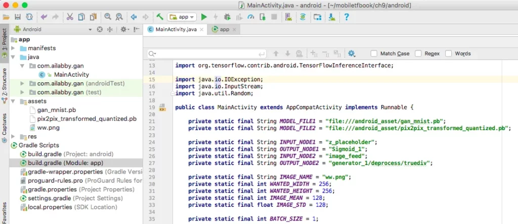
Now, we’ll create a few instance variables:
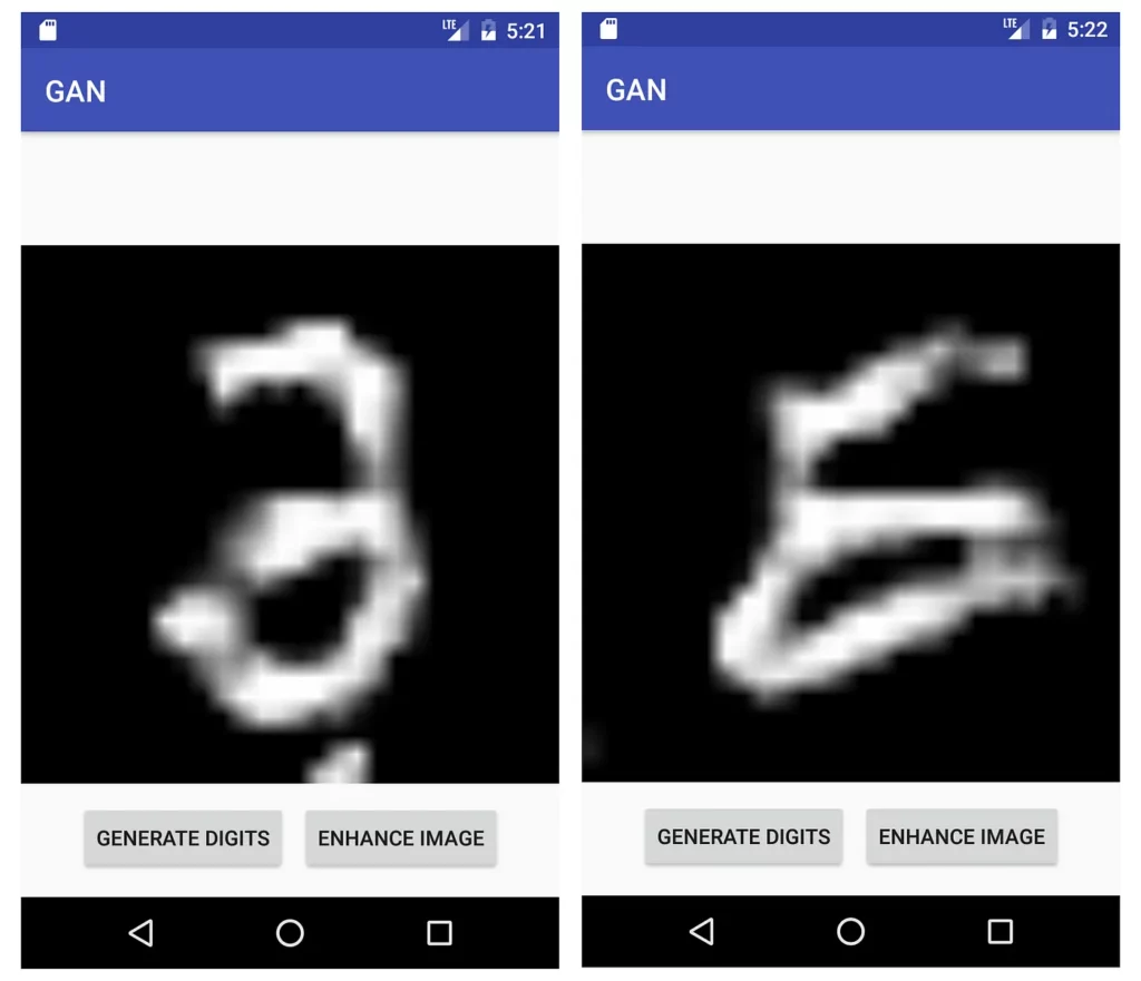
The app layout consists of one ImageView and two buttons. The first button will help us generate a random number image using our gan_mnist.pb model. And the second button will help enhance the image.
Then, we set up two click listeners for the two buttons:
When a button is tapped, the run method runs in a worker thread:
In the runMNISTModel method, we first prepare a random input to the model:
Then we feed the input to the model, run the model, and get the output values, which are scaled grayscale values between 0.0 and 1.0. We then convert those values to integers in the range of 0 and 255:
After that, we use the returned and converted grayscale values for each pixel that gets set when creating a bitmap:
Finally, we show the bitmap in the main UI thread’s ImageView:
If you run the app now, you’ll see the initial screen and the result after you tap GENERATE DIGITS as in Figure below:
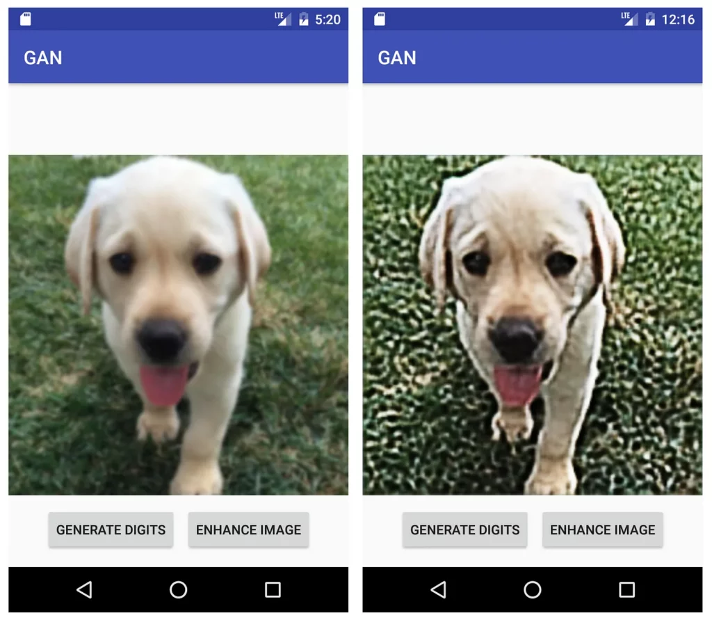
Now, let’s use the Enhance Image function—for that, we will take an image that’s a bit blurry and will try to see the effect of enhancing it with pix2pix.
Run the app again and tap the ENHANCE IMAGE button. Now, you’ll see in a few seconds the enhanced image, similar to below:
Final Takeaway
GANs require very high-end computational power and massive amounts of data to train. Here is an example of a GAN in action; this GANs model was trained for a long time and with very high-end processing power.
I would also say that this is the kind of accuracy we all want with GANs. Currently, we have many pre-trained GANs models provided by big organizations. But this is just a small portion of GANs—we can use GANs for text, and with smaller-sized datasets.
Moving forward, it will be interesting to see how we’ll be able to utilize GANs on devices with limited computational power.

I hope you liked this piece! See you in the next article.

Comments 0 Responses