This post gives an overview of the different techniques for how to handle categorical variable encoding—i.e. permanently replacing category strings with numerical representations.
Table of contents:
Categorical Encoding
Most machine learning algorithms and deep neural networks require numerical inputs. This means that if we have categorical data, we must first encode it to numbers in order to build models that actually work.
Simply put, the goal of categorical encoding is to produce variables we can use to train machine learning models and build predictive features from categories.
In this post, we present a number of techniques for this kind of data transformation; here is a list of the different techniques:
Traditional techniques
- One-hot encoding
- Count or frequency encoding
- Ordinal or label encoding
Monotonic relationship
- Ordered label encoding
- Mean encoding
- Probability ratio encoding
- Weight of evidence
Alternative techniques
- Rare labels encoding
- Binary encoding
To get started, we need to install a library called category_encoders, which contains a lot of basic and advanced methods for categorical variable encoding. Here’s how you can install it in your environment:
We’re going to use the following sample data to demonstrate the methods:

One-hot encoding
One-hot encoding consists of encoding each categorical variable with a set of boolean variables that take values of 0 or 1. This value then serves to indicate if a category is present for each observation.
There are multiple variants of this technique:
One-hot encoding into k-1 variables
We can one-hot encode a categorical variable by creating k-1 binary variables, where k is the number of distinct categories.
One-hot encoding into k-1 binary variables allows us to use one less dimension and still represent the data fully.
Take, for example, the case of binary variables like a medical test. Where k=2 (positive/negative), we need to create only one (k -1 = 1) binary variable.
Most machine learning algorithms consider the entire dataset while training. Therefore, encoding categorical variables into k-1 binary variables is better, as it avoids introducing redundant information.
One-hot encoding into k variables
There are a few occasions when it’s better to encode variables into k variables:
- When building tree-based algorithms.
- When making feature selection with recursive algorithms.
- When interested in determining the importance of every single category.
Here is an illustration of one-hot encoding into k variables:

One-hot encoding of most frequent categories
When performing one-hot encoding, we can only consider the most frequent categories ( the categories that have high cardinality) in a variable. This helps us avoid overextending the feature space.
Advantages of one-hot encoding
- Does not assume the distribution of categories of the categorical variable.
- Keeps all the information of the categorical variable.
- Suitable for linear models.
Limitations of one-hot encoding
- Expands the feature space.
- Does not add extra information while encoding.
- Many dummy variables may be identical, and this can introduce redundant information.
Finally, here is a code snippet with the Pandas library to achieve k and k-1 one-hot encoding:
# import the pandas library
import pandas as pd

# read your dataset
data = pd.read_csv("yourData.csv")

# perform one hot encoding with k
data_with_k = pd.get_dummies(data)

# perform one hot encoding with k - 1, it automatically drop the first.
data_with_k_one = pd.get_dummies(data, drop_first = true)
Integer (Label) Encoding
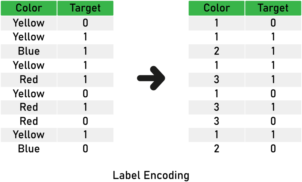
Integer encoding (also known as label encoding) includes replacing the categories with digits from 1 to n (or 0 to n-1, depending on the implementation), where n is the number of the variable’s distinct categories (the cardinality), and these numbers are assigned arbitrarily.
Here’s an illustration of the concept:

Advantages of integer (label) encoding
- Straightforward to implement.
- Does not expand the feature space.
- Can work well enough with tree-based algorithms.
- Allows agile benchmarking of machine learning models.
Limitations of integer (label) encoding
- Does not add extra information while encoding.
- Not suitable for linear models.
- Does not handle new categories in the test set automatically.
- Creates an order relationship between the categories.
Here’s a code snippet to do the integer encoding:
# the pandas library
import pandas as pd

# get you data
data = pd.read_csv("yourData.csv")

# function to find the different enumuration of variable.
def create_category_mapping(data, variable):
    return {k: i for i, k in enumerate(data[variable].unique(), 0)}

# function to apply the encoding on the variable.
def label_encode(train, test, variable, ordinal_mapping):
    train[variable] = train[variable].map(ordinal_mapping)
    test[variable] = test[variable].map(ordinal_mapping)

# check that data contains only
for variable in data.columns:
    mappings = create_category_mapping(data, variable)
    label_encode(train, test, variable, mappings)
Count or Frequency Encoding
Here, we replace categories with the count or percentage of observations that show each category in the dataset. Thus, we capture the representation of each label in the dataset.
Here’s an illustration of this method:

What this technique assumes is that the number of observations are informative of the category’s predictive power.
Advantages of Count or Frequency encoding
- Straightforward to implement.
- Does not expand the feature space.
- Can work well with tree-based algorithms.
Limitations of Count or Frequency encoding
- Not suitable for linear models.
- Does not handle new categories in the test set automatically.
- We can lose valuable information if there are two different categories with the same amount of observations count—this is because we replace them with the same number.
Here’s the code snippet for this method with Pandas:
# import the pandas library.
import pandas as pd

# get you data
data = pd.read_csv("yourData.csv")

# loop to find the different count of categories in a dict and apply them to the variable
# in train and test set.
for variable in train.columns:
    count_dict = train[variable].value_counts().to_dict()
    train[variable].map(count_map)
    test[variable].map(count_map)
Ordered Label Encoding
This method replaces categories with integers from 1 to n, where n is the number of distinct categories in the variable (the cardinality). However, we use the target mean information of each category to decide how to assign these numbers.
Here’s a detailed illustration of this technique:

Advantages of ordered label encoding
- Straightforward to implement.
- Does not expand the feature space.
- Creates a monotonic relationship between categories and the target.
Limitations of ordered label encoding
- It may lead to overfitting.
Here’s the code for ordered label encoding with Pandas:
# import the pandas library.
import pandas as pd

# get you data.
data = pd.read_csv("yourData.csv")

# get your target variable name.
target = "your target variable name"

# we generate the order list of labels, then apply it to the variable.
for variable in train.columns:
    labels = train.groupby([variable])[target].mean().sort_values().index
    mapping = {x: i for i, x in enumerate(labels, 0)}
    # apply the encoding to the train and test sets.
    train[variable] = train[variable].map(mapping)
    test[variable] = test[variable].map(mapping)
Mean (Target) Encoding
Mean encoding means replacing the category with the mean target value for that category.
We start by grouping each category alone, and for each group, we calculate the mean of the target in the corresponding observations. Then we assign that mean to that category. Thus, we encoded the category with the mean of the target.
Here’s a detailed illustration of mean encoding:

Advantages of Mean encoding
- Straightforward to implement.
- Does not expand the feature space.
- Creates a monotonic relationship between categories and the target.
Limitations of Mean encoding
- May lead to overfitting.
- May lead to a possible loss of value if two categories have the same mean as the target—in these cases, the same number replaces the original.
To apply this technique, you can use the following code:
# import the pandas library.
import pandas as pd

# get you data.
data = pd.read_csv("yourData.csv")

# get your target variable name.
target = "your target variable name"

# loop over the categorical columns to apply the encoding.
for variable in train.columns:
    # create dictionary of category:mean values.
    dict = train.groupby([variable])[target].mean().to_dict()
    # apply the encoding to the train and test sets.
    train[variable] = train[variable].map(dict)
    test[variable] = test[variable].map(dict)
Weight of Evidence Encoding
Weight of evidence (WOE) is a technique used to encode categorical variables for classification.
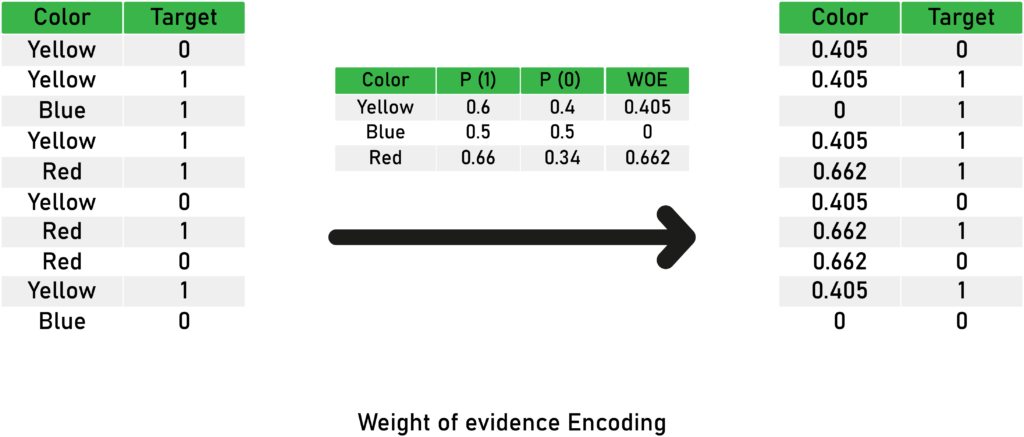
The rule is simple; WOE is the natural logarithm (ln) of the probability that the target equals 1 divided by the probability of the target equals 0.
Here is a mathematic formula : WOE = ln (p(1) / p(0)).
- Where p(1) is the probability of the target being 1, and p(0) is the probability of the target being 0.
The WOE is bigger than 0 if the probability of the target being 0 is more significant and smaller than 0 when the probability of the target being 1 is more significant.
This way, the WOE transformation creates an excellent visual representation of the variable. By looking at the WOE encoded variable, you can see which category favors the target being 0 or 1.
Here’s a detailed illustration of the concepts behind WOE:

Advantages of the Weight of evidence encoding
- Creates a monotonic relationship between the target and the variables.
- Orders the categories on a “logistic” scale, which is natural for logistic regression.
- We can compare the transformed variables because they are on the same scale. Therefore, it’s possible to determine which one is more predictive.
Limitations of the Weight of evidence encoding
- May lead to overfitting.
- Not defined when the denominator is 0.
Here’s a code snippet using Pandas and NumPy:
# import the pandas and numpy libraries.
import pandas as pd
import numpy as np

# get you data.
data = pd.read_csv("yourData.csv")

# get your target variable name.
target = "your target variable name"

# we loop over all the categorical variables
for variable in train.columns:

    # calculating the mean of target for each category. (probability of events or p(1))
    dataframe = pd.DataFrame(train.groupby([variable])[target].mean())

    # calculating the non target probability. (probability of non-events or p(0))
    dataframe['non-target'] = 1 - dataframe[target]

    # calculating the WOE.
    dataframe['ratio'] = np.log(dataframe[target] / dataframe['non-target'])
    ratio_mapping = dataframe['ratio'].to_dict()

    # applying the WOE.
    train[variable] = train[variable].map(ratio_mapping)
    test[variable] = test[variable].map(ratio_mapping)
Probability Ratio Encoding
This encoding is suitable for classification problems only, where the target is binary.
It’s similar to WOE, but we don’t apply the natural logarithm. Instead, for each category, we calculate the mean of the target = 1, which is the probability of the target being 1 (P(1)), and the probability of the target being 0 (P(0)).
Finally, we calculate the ratio = P(1)/P(0), and we replace the categories by that ratio.
Here’s a simple illustration to demonstrate the concept:

Advantages of probability ratio encoding
- Captures information within the category, and therefore creates more predictive features.
- Creates a monotonic relationship between the variables and the target. So it’s suitable for linear models.
- Does not expand the feature space.
Limitations of probability ratio encoding
- Likely to cause overfitting.
- Not defined when the denominator is 0.
Here’s a code snippet using Pandas and NumPy:
# import the pandas and numpy libraries.
import pandas as pd
import numpy as np

# get you data.
data = pd.read_csv("yourData.csv")

# get your target variable name.
target = "your target variable name"

# we loop over all the categorical variables
for variable in train.columns:

    # calculating the mean of target for each category. (probability of events or p(1))
    dataframe = pd.DataFrame(train.groupby([variable])[target].mean())

    # calculating the non target probability. (probability of non-events or p(0))
    dataframe['non-target'] = 1 - dataframe[target]

    # calculating the ration.
    dataframe['ratio'] = dataframe[target] / dataframe['non-target']
    ratio_mapping = dataframe['ratio'].to_dict()

    # applying the probability ration encoding.
    train[variable] = train[variable].map(ratio_mapping)
    test[variable] = test[variable].map(ratio_mapping)
Rare Label Encoding
Rare labels are those that appear only in a tiny proportion of the observations in a dataset. Rare labels may cause some issues, especially with overfitting and generalization.
The solution to that problem is to group those rare labels into a new category like other or rare—this way, the possible issues can be prevented.
Here’s an illustration of rare labels grouped into others label:

This way, categories that are new in the test set are treated as rare, and the model can know how to handle those categories as well, even though they weren’t present in the train set.
Here’s a code snippet:
# import the pandas and numpy libraries.
import pandas as pd
import numpy as np

# get you data.
data = pd.read_csv("yourData.csv")

# define your threshold here
threshlold = 0.05

# we loop over all the categorical variables
for variable in train.columns:

    # locate all the categories that are not rare.
    counts = train.groupby([variable])[variable].count() / len(train)
    frequent_labels = [x for x in counts.loc[counts>threshlold].index.values]

    # change the rare category names with the word rare, and thus encoding it.
    train[variable] = np.where(train[variable].isin(frequent_labels), train[variable], 'Rare')
test[variable] = np.where(test[variable].isin(frequent_labels), test[variable], 'Rare')- You should set up a threshold percentage value, under which you consider if a label is rare or not.
Binary encoding
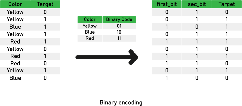
The binary encoding uses (as its name indicates) binary code; the process is relatively easy and straightforward. As a first step, we convert each integer to binary code. Then each binary digit gets one column in the dataset.
If there are n unique categories, then binary encoding results in the only log base 2 of n features, which is = ln(n) / ln(2)
Advantages of Binary encoding
- Straightforward to implement.
- Does not expand the feature space too much.
Limitations of Binary encoding
- It exposes the loss of information during encoding.
- It lacks the human-readable sense.
Here’s an illustration of the binary encoding technique:

And here’s code snippet using Category Encoders library:
# import the libraries
import pandas as pd
from category_encoders import BinaryEncoder

# get your data.
data = # your data

# split into X and y.
x_train = data.drop('target', axis = 1)
y_train = data['target']

# create an encoder object - it will apply on all strings columns.
binary = BinaryEncoder()

# fit and transform to get encoded data.
binary.fit_transform(x_train, y_train)
Conclusion
That was so much information to absorb in one article. To recap simply, the idea is to change the encoding of a given categorical variable to something better for the machine learning model.
We explored plenty of methods in this post, and you can try out different approaches to the problem to see which ones provide more reliable results.
There are other advanced methods out there; I recommend checking out the category encoders documentation to learn more about them.

Comments 0 Responses