Compression involves processing an image to reduce its size so that it occupies less space. There are already codecs, such as JPEG and PNG, whose aim is to reduce image sizes. There are two types of image compression; lossy and lossless.
In lossless compression, one can retrieve the original image data, while in lossy compression one cannot. As a point of reference, PNG is lossless and JPEG is lossy.
Image compression is very crucial in order to reduce the size of disk space used as well as reduce the amount of internet bandwidth used while loading images. It’s also important to compress images for people accessing the internet via low bandwidth connections.
In this article, we’ll look at how deep learning can be used to compress images in order to improve performance when working with image data.
We’ll now look at some research that’s been conducted in an attempt to solve this problem:
- Five Modulus Method (FMM) for Image Compression
- Variable Rate Image Compression with Recurrent Neural Networks
- End-to-end Optimized Image Compression
- Full Resolution Image Compression with Recurrent Neural Networks
- Lossy Image Compression with Comprehensive Autoencoder
- Semantic Perceptual Image Compression using Deep Convolution Networks
- An End-to-End Compression Framework Based on Convolutional Neural Networks
- CocoNet: A Deep Neural Network for Mapping Pixel Coordinates to Color Values
- And the Bit Goes Down: Revisiting the Quantization of Neural Networks
Five Modulus Method (FMM) for Image Compression (2012)
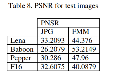
The authors of this paper are from the Irbid National University and Toledo College. The FMM method involves converting each pixel value in an 8 X 8 block into a multiple of 5 for each of the RGB arrays. The new values are then divided by 5 to obtain new values that are of 6-bit length for every pixel. This 6-bit pixel has less storage space compared to the 8-bit length pixel.
The FMM algorithm is designed to check the whole pixel in the 8 x 8 and covert each pixel to a number divisible by 5, based on the conditions below:

A(i,j) is the digital representation of the 8 x 8 block for the RGB arrays. The table below shows the transformations.

The obtained numbers are divided by 5 again to give a remainder between 0 and 51. The metric used for tests is the peak signal-to-noise ratio (PSNR). The results shown below suggest that this model isn’t optimal for image compression; it can, however, be added to existing solutions.


Variable Rate Image Compression with Recurrent Neural Networks (ICLR, 2016)
The authors of this paper are from Google. This paper proposes a framework for variable-rate image compression and an architecture based on convolutional and deconvolutional LSTM recurrent networks for increasing thumbnail compression. This LSTM-based approach provides better visual quality than JPEG, JPEG2000, and WebP. It reduces storage size by at least 10%.
This paper is primarily based on a class of neural networks known as autoencoders. A compression autoencoder usually has three parts:
- an encoder that takes in an image and converts it into
- a bottleneck (usually a flat neural net layer) that represents the compressed data that’s then transformed by
- a decoder into a figure that resembles the original image
The bottleneck allows for the visual fidelity and compression rate of the encoded image to be controlled by changing the number of nodes in this layer. For every architecture described in this paper, a function E takes an input image and emits an encoded version. This is then processed by a binarization function B. A decoder function D takes the binary version and outputs a reconstructed version. These three components form an autoencoder, which is used in all compression networks.
In a feed-forward, fully-connected residual encoder, the authors set E and D to be composed of a fully-stacked connected layer. In the LSTM-based approach, the authors use LSTM models for the decoder and autoencoder. E and D are made up of stacked LSTM layers.


For the encoder, the authors use one fully-connected layer followed by two stacked LSTM layers. For the decoder, they use two stacked LSTM layers followed by a fully-connected layer with a tanh nonlinearity that predicts RGB values.
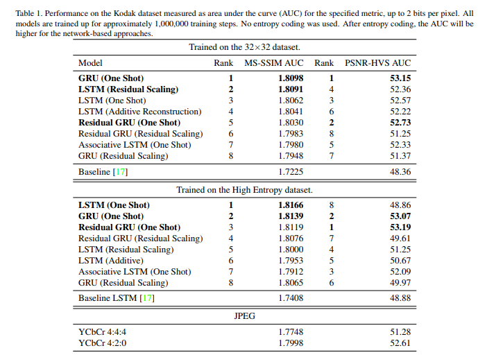
For evaluation, the authors use the Structural Similarity Index (SSIM). Their 32×32 benchmark dataset has 216 million random color images collected from the internet. The figure below shows the performance of their models.

End-to-end Optimized Image Compression (ICLR, 2017)
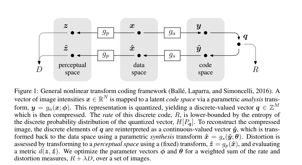
The authors of this paper are from New York University. This paper describes an image compression method made up of nonlinear analysis transformation, a uniform quantizer, and a nonlinear synthesis transformation. The transformations consist of three convolutional linear filters and nonlinear activation functions that follow each other.
As shown below, the authors have created a method for end-to-end optimization of an image compression model based on nonlinear transforms. They use generalized divisive normalization (GDN) joint nonlinearity that is inspired by the neurons in biological visual systems.
This transformation is followed by a uniform scalar quantization where each element is rounded off to the nearest integer. Reconstructing the image is then done from the quantized values using an approximate parametric nonlinear inverse transformation.

In the presence of quantization, stochastic gradient descent produces zero gradients almost everywhere. To solve this problem, the authors use a proxy loss function that’s based on a continuous relaxation of the probability model. This replaces the quantization step with additive uniform noise.

Full Resolution Image Compression with Recurrent Neural Networks (CVPR, 2017)
The authors of this paper are from Google. This paper presents a set of full-resolution lossy image compression methods based on neural networks. The authors’ aim is to come up with a new network that performs well on the task of compressing images of any size.

The architectures consist of a recurrent neural network-based encoder and decoder, a binarizer, and a neural network for entropy encoding. The authors achieve a 4.3%–8.8% AUC (area under the rate-distortion curve) improvement. Their neural network outperforms JPEG on the rate-distortion curve on the Kodak dataset images, with and without the aid of entropy coding.
The compression network is composed of an encoding network E, a binarizer B and a decoding network D. E and D contain recurrent network components. Images are first encoded and then transformed into binary codes that are stored or fed to the decoder. Using the received codes, the decoder network creates a representation of the original image.

For evaluation, the authors use the Multi-Scale Structural Similarity (MS-SSIM) and the Peak Signal-to-Noise Ratio — Human Visual System (PSNR-HVS).

Lossy Image Compression with Comprehensive Autoencoder (2017)
The authors of this paper are from Twitter. They propose a way to optimize autoencoders for lossy image compression.
The authors define a compressive autoencoder (CAE) with three components: an encoder f, a decoder g, and a probabilistic model Q. In the first two layers of the model, the encoder performs mirror padding and a fixed pixelwise normalization. The padding is done in such a manner that the output of the encoder will have the same spatial extent as a times downsampled image.
The purpose of the normalization is to center the distribution of each channel’s value and make sure that it’s of unit variance. Thereafter, the image is convolved and spatially downsampled while increasing the number of channels to 128. This is accompanied by three residual blocks. Each block has two convolutional layers with 128 filters each.

After this, a final convolutional layer is applied and the coefficients are downsampled. Quantization is then applied by rounding to the nearest integer. The architecture uses zero-padded convolutions.
Upsampling occurs through convolution and a reorganization of the coefficients, which turns a tensor that has many channels into a tensor of the same dimensionality. This tensor, however, has fewer channels and a larger spatial extent. A sub-pixel convolution layer is then formed from the convolution and reorganization of the coefficients. The three residual blocks and two sub-pixel layers upsample the image to the resolution of the input. The values of the pixels are then clipped between 0 to 255 after denormalization.

Semantic Perceptual Image Compression using Deep Convolution Networks (DCC, 2017)
This paper has been written by authors from Brandeis University. They present a CNN aimed at semantic image understanding to achieve higher visual quality in lossy compression focussed on JPEG. Experiments are tested on the Kodak PhotoCD dataset and the MIT Saliency Benchmark dataset.
Their model improves the visual quality of JPEG by using a higher bit rate to encode image regions flagged by their model as having content of interest, and lowering the bits in other regions in the image.
The model has an advanced JPEG encoder that enables the quantization of every region to be decided by the knowledge of the image content. The visual quality is improved by improving the signal-to-noise ratio with multiple regions of interest. The final JPEG encoding produced can be decoded with any standard JPEG decoder. The authors evaluate their model on the PSNR metric, structural similarity (SSIM) and MS-SSIM for JPEG and JPEG2000.

The model was trained on the Caltech-256 dataset. The figure below shows some of the results obtained on KODAK images and a comparison on different metrics.


An End-to-End Compression Framework Based on Convolutional Neural Networks (2017)
This paper has been drafted by researchers from IEEE. The paper proposes the integration of two CNNs into an end-to-end compression framework. They have focused their efforts on image compression, image denoising, image resampling, image restoration, and image completion.
The proposed compression framework is compatible with existing image codecs such as JPEG, JPEG2000, and BPG. Their first CNN is named compact convolutional neural network (ComCNN) and the second reconstruction convolutional neural network (RecCNN).

ComCNN learns optimal compact representation from an input image, which is then decoded using an image codec such as JPEG. The RecCNN reconstructs the decoded image at high quality.

The ComCNN has three weight layers that maintain the spatial structure of the original image and enable for perfect reconstruction. This network uses the ReLu activation function. 64 filters of size 3 x 3 x c are used to generate 64 feature maps, where c is the number of image channels.
RecCNN has 20 weight layers which consist of convolution + ReLU, convolution + batch normalization + ReLU and convolution layers. In the first layer, 64 filters of size 3 x 3 x c are used to generate 64 feature maps. ReLu activation then follows. From layer 2 to 19, 64 filters of sizes 3 x 3 x 64 are used, adding batch normalization between convolution and ReLU. In the last layer, c filters of size 3 x 3 x 64 are used to reconstruct the output image.
In order to speed up learning and boost performance, residual learning and batch normalization is applied. Upsampling the compressed image to the original image is done using bicubic interpolation. The figure below shows the performance of the method in comparison to other compression algorithms such as JPEG.

CocoNet: A Deep Neural Network for Mapping Pixel Coordinates to Color Values (ICNIP, 2018)
This paper proposes a deep neural network that maps the 2D pixel coordinates of an image to the corresponding RGB color values. The network named CocoNet stands for coordinates-to-color network.
During the training process, the network learns a continuous function that’s able to approximate the discrete RGB values that have been sampled over the discrete 2D pixel locations. Using every 2D pixel location, the network is able to reconstruct the entire image. In this model, an individual neural network is trained for each input image, meaning that one network encodes one image only.

The CocoNet beats other image denoising methods on the CIFAR-10 dataset. This also obtains better upsampling results compared to bicubic interpolation. The figure below shows the performance of the model on various metrics.


And the Bit Goes Down: Revisiting the Quantization of Neural Networks (2019)
This is a relatively new paper from Facebook AI Research. This paper tackles the problem of reducing the memory footprint of ResNet-like convolutional network architectures. The authors introduce a vector quantization method whose aim is to preserve the quality of the reconstruction of the network outputs and not the weights. The approach proposed in this paper doesn’t require the use of labeled data.

This approach achieves a 76.1 top-1 accuracy when applied to the semi-supervised ResNet-50 ImageNet object classification task. The model is comprised of a fully-connected layer that’s applied to a convolution layer.
The model uses Product Quantization (PQ) in order to take advantage of the high correlation in convolutions, and it uses an alternative PQ that directly minimizes the reconstruction error. Network quantization is done sequentially from the lowest layer to the highest.
During experimentation, the authors quantize the vanilla ResNet-18 and ResNet-50 architectures, pre-trained on the ImageNet dataset. The pre-trained models are largely obtained from the PyTorch model zoo. For evaluation, the authors mainly focus on memory and accuracy.

The model is evaluated on the ImageNet benchmark for ResNet-18 and ResNet-50 architectures. The figure below is a comparative representation of the results obtained.

Conclusion
We should now be up to speed on some of the most common — and a couple of very recent — techniques for performing deep learning-based compression in a variety of contexts.
The papers/abstracts mentioned and linked to above also contain links to their code implementations. We’d be happy to see the results you obtain after testing them.

Comments 0 Responses