A guide to the top machine learning algorithms

The world is currently generating 2.5 quintillions of data each day, according to Forbes. The power of deriving meaning from these loads of data relies on the use of specialized machine learning algorithms that have been developed over time. We can teach machines to learn—or they can learn on their own.

What is machine learning all about?

At its core, machine learning is about creating algorithms (sets of rules) that learn complex functions or patterns from data to make predictions.

Each machine learning algorithm has its own strengths and weaknesses. Some models are easier to understand or interpret but lack predictive power, while others have accurate predictions but lack interpretability.

Broadly speaking, machine learning is best suited for:

• Gleaning insights about complex problems and huge amounts of data.
• Problems for which existing solutions require a long list of rules (or constantly fine-tuning the rules); ML algorithms can simplify these existing solutions.
• Dynamic environments, where new data is regularly created. Machine learning algorithms can adapt to these new environments.

This article will provide an overview of how some of the top and most commonly-used ML algorithms work, their strengths and drawbacks, and their implementation using Python.

Machine learning algorithms can be classified as:

• Supervised algorithms
• Unsupervised algorithms
• Reinforcement learning

Supervised Machine Learning Algorithms

The input data for supervised machine learning algorithms are labeled by humans, and the output is known and accurate. Depending on what you want to predict, supervised learning can be used to solve two types of problems:

i. Regression Problems

Used to predict continuous values, such as market forecasts, life expectancy, and population growth.

ii. Classification Problems

Used when you want to predict a discrete or categorical variable, such as high or low stock prices, or a binary classification problem with a yes or no (either/or) answer.

Unsupervised Machine Learning Algorithms

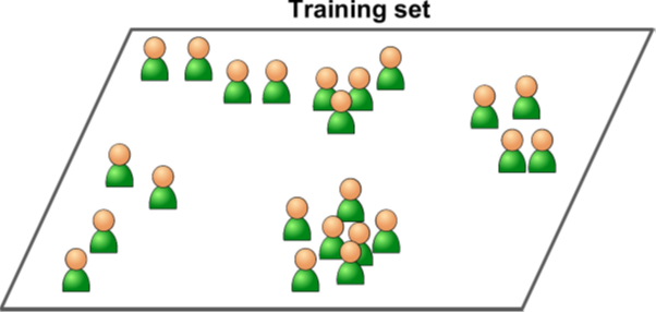
With unsupervised algorithms, machines/computers try to learn on their own by detecting patterns in data and grouping those patterns for analysis. There is no labeled data.

Unsupervised learning groups data by:

i. Clustering

Clustering techniques look for similarities in the data. If there are similarities, then clustering algorithms categorize the data in certain ways. This kind of algorithm is used in customer and product segmentation for target marketing.

ii. Association

Association techniques try to understand the rules and meanings behind different groups. A common example is finding the relationship between customer purchases, such as products that are purchased concurrently in a superstore.

Reinforcement Learning

Reinforcement learning works on a reward/penalty concept. The machine/computer is rewarded when it learns correctly and penalized when it learns incorrectly. The learning process is iterative, and the machine improves with each subsequent iteration. Examples of reinforcement learning include self-driving cars or game-based tasks like analyzing/predicting moves in Chess or Go.

We’ll now dive into the individual ML algorithms, their applications, advantages, disadvantages, and Python implementations.

Linear Regression

Linear regression is used to understand the linear relationship between a dependent and independent variable, and how change in one variable impacts the other. The relationship can either be positive, negative or neutral. The independent variable is explanatory, as it explains the factors that impact the dependent variable. The dependent variable is the predictor.

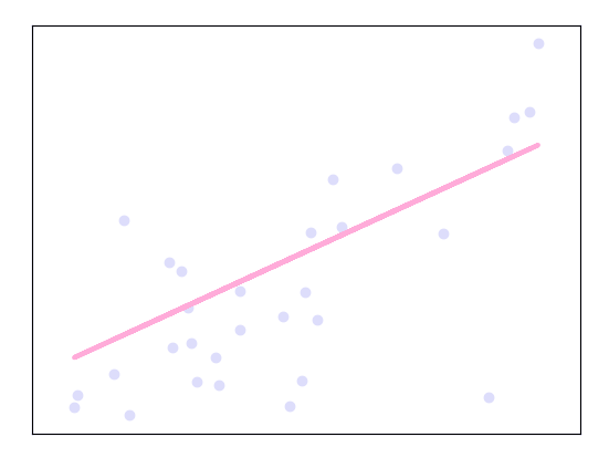
Mathematically, the linear relationship between the dependent and independent variable can be written as:

Y = β0 + β1X

Where Y is the dependent variable, X is the independent variable, and β1 and β0 are unknown constants that represent the slope and intercept, respectively.

We use training data to determine the estimates of β1 and β0 by drawing a line of best fit. We’ll then use β1 and β0 coefficients for predictions on the test data.

Linear Regression is grouped into a couple of different categories, which we’ll explore below:

i. Simple linear regression

Based on the value of a single explanatory/independent variable, the value of the dependent variable changes.

Y = β0 + β1X0

ii. Multiple linear regression

The response variable is dependent on more than one explanatory variable.

Y = β0 + β1X0 + β2X1

What are the advantages of linear regression?

1. It is best suited for linear relationships.
2. It is very fast to implement, easy to understand, and less prone to overfitting.

What are the disadvantages of linear regression?

1. Linear regression performs poorly on non-linear relationships.

Linear models work on the assumption that the relationship between the response and the predictor variable is linear. If the true relationship is far from linear, then all the insights obtained from the model fit is wrong. Furthermore, the prediction accuracy of the model is significantly reduced.

Applications

• Sale Estimation — Commonly used in the business sector for sale forecasting based on explanatory variables such as advertising cost and product price.
• Risk Assessment — Applicable to the insurance or financial domains to assess risk levels involved and to help make informed decisions on those risks.

Python Implementation

#python code for Linear Regression
from sklearn.linear_model import LinearRegression
lin_reg=LinearRegression()
model=line_reg.fit(X,y)
predicted=model.predict(X_new)

Scikit-learn and statsmodel Python libraries are used for implementing linear regression:

Logistic Regression

Logistic regression is commonly used to estimate the probability that an instance belongs to a particular class—i.e. what is the probability that this email is spam?

f the estimated probability is greater than 50%, then the model predicts that the instance belongs to the positive class labeled “1”. Otherwise, it predicts that it doesn’t and belongs to the negative class labeled “0”. This makes the model a binary classifier.

Logistic regression models compute the weighted sum of input features, but instead of outputting the results directly, they outputs the logistic result.

This can be expressed mathematically as:

The left-hand side is the logit or log-odds function, and p(X)/ 1-p(x) is the odds.

Logistic regression can be classified into 3 types based on the nature of the categorical response:

i. Binary logistic regression

Used when the categorical response has two possible outcomes, such as yes or no. Examples include predicting whether a cell is cancerous or not, or whether a team will win or lose.

ii. Multi-nominal logistic regression

The categorical response has three or more possible outcomes with no ordering, such as predicting commonly-used programming languages (SQL, Python, Java, C++, JavaScript)

iii. Ordinal logistic regression

The categorical response has three or more possible outcomes with natural ordering. An example is how a customer rates service quality in a superstore on a scale of 1 to 10.

When should one use logistic regression?

i. When classifying elements into two categories based on the explanatory variable; i.e. classify defaulters and non-defaulters based on their repayment histories.

ii. When there is a need to predict probabilities that the categorical dependent variable will fall into two categories of the binary response as a function of the explanatory variable—i.e. what is the probability a politician will be elected based on their campaign policies?

What are the advantages of using logistic regression?

1. Easy to interpret and less prone to overfitting.
2. Controls confounding and tests interaction.
3. Can handle non-linear effects.

What are the disadvantages of using logistic regression?

1. Requires more data to achieve stability and meaningful results.
2. Not robust to outliers and missing values.
3. When the training data is sparse and high dimensional, the model may overfit the training data.

Applications of Logistic Regression

• In weather forecasting to predict the probability of weather conditions (rainy, windy, cloudy).
• In credit scoring systems for risk management i.e. if a customer will default a loan.
• In election forecasting to predict whether a candidate will win or lose an election.

Python Implementation

# Python code for Logistic Regression
#Import LogisticRegression model
from sklearn.linear_model import LogisticRegression
#create logistic regression
log_reg = LogisticRegression()
#fit model to the training dataset
model=log_reg.fit(X,y)
#predict output
predicted = model.predict(X_new)

Naïve Bayes Classifier

Naïve Bayes classifiers work on the popular Bayes Theorem of probability. They assume independence between the predictors.

Consider a given shape—a rectangle based on the number of edges and vertices. The classifier assumes all these characteristics independently contribute to the probability of the shape being rectangular. This is despite the features being dependent on each other.

When do we use a Naïve Bayes classifier?

i. With very large or moderate datasets.

ii. If the instances have several attributes.

What are the advantages of Naïve Bayes classifiers?

1. Perform well when the input variables are categorical.
2. Very simple and perform better than many highly-sophisticated classification methods.
3. Converge faster, hence require little training data as compared to other discriminative methods like logistic regression.

Applications of Naïve Bayes classifiers

• Building classification models for different disease predictions.
• News topic classification into either technology, sports, entertainment.
• Email spam filtering — Gmail uses a Naïve Bayes classifier to group our emails as either spam or not.
• Sentiment analysis —group comment reviews as positive, negative, or neutral.

Python Implementation

#Import Gaussian Naive Bayes model
from sklearn.naive_bayes import GaussianNB
#Create a Gaussian Classifier
model= GaussianNB()
# Train the model using the training sets
model.fit(features,label)
#Predict Output
predicted= model.predict(label_new)

K-Means Clustering

K-means clustering is an unsupervised algorithm used for cluster analysis.

It’s an iterative algorithm that partitions a group of data containing n values into k clusters or subgroups, with each of the n values belonging to the k cluster with the nearest mean.

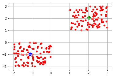
K-means clustering operates on a given dataset through a predefined number of k-clusters. The clusters of data are grouped based on their similarities and the distance of each data point in the cluster with the mean of their centroid.

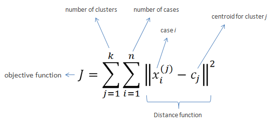
K-means clustering also tends to minimize the Euclidean distance that each point has from the centroid of the cluster. This is the intra-cluster variance and can be minimized using the squared error function, as shown below:

K-means clustering process

1. We randomly initialize and select k points (k=4).
2. We use the Euclidean distance to find the data points closest to the center of the cluster.
3. We calculate the mean of all points in the cluster, which is their centroid.
4. We iterate on steps 1 to 3 until all the data points have been assigned to their respective clusters.

What are the advantages of K-Means Clustering?

1. If k is a smaller value, k-means computes faster than hierarchical clustering for a large number of variables.
2. In the case of globular clusters, K-means produces tighter clusters than hierarchical clustering.

Applications of K-means clustering

• Document clustering to find relevant documents.
• Used by most search engines such as Google to cluster web pages by similarity and identify the relevance of said search results.
• In the business sector, it’s used to identify segments of purchases made by customers.

Python Implementation

from sklearn.Cluster import KMeans
#initialize k with 3
model=KMeans(n_Clusters=3)
#fit model to train data
Kmean_cluster=model.fit(x)
#obtain centroid
Kmean_cluster.cluster_centers_
Kmean_cluster.predict(x_test)

Support Vector Machine

Support vector machine is a supervised ML algorithm for classification or regression problems. SVM works by classifying data into different classes by plotting a line (hyperplane) that separates the training data set into classes.

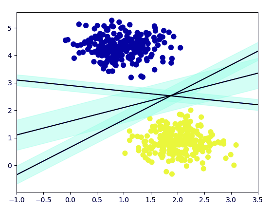
SVM aims to maximize the distance between the various classes or groups involved. This is known as margin maximization and ensures that the closest point in each class lies furthest from each other.

When the hyperplane that maximizes the distance between the classes has been identified, then the probability to generalize well to unseen data increases.

Let’s break down the SVM algorithm to have a better understanding of how it works:

S — Support refers to the extreme values in your dataset.

V — Vectors are the values or data points.

M — Machine is the ML algorithm that focuses on support vectors to classify groups or classes of data. The algorithm focuses on the extreme points ignoring the rest of the dataset.

SVM algorithms are classified into 2 categories:

i. Linear Support Vector Machine

This is where the training data are separated by the hyperplane.

ii. Non-Linear Support Vector Machine

With non-linear SVMs, it isn’t possible to separate the training data using a hyperplane. In such situations, the training data is usually too complex, making it impossible to find a representation for every feature vector, i.e. linearly separating a set of face images from non-faces.

What are the advantages of SVM?

1. Doesn’t make any strong assumptions on the data.
2. Renders more efficiently for correct classification of the feature data
3. SVM offers the best classification performance on training data
4. It doesn’t overfit the data

What are the disadvantages of SVM?

1. SVM is hard to interpret and requires a lot of memory and processing power.
2. It doesn’t provide probability estimations and is sensitive to outliers.

Applications of SVM

SVM is commonly used for stock market forecasting by various financial institutions, such as to compare the performance of two stocks within the same sector.

Python Implementation

#python code for implementation.
from sklearn.svm import SVC
svm_model = SVC(kernel=’rbf’)
svm_model.fit(X,y)
predicted = svm_model.predict(X_new)

Apriori Algorithm

Apriori is an unsupervised ML algorithm that generates underlying relations or association rules from a given dataset.

The association rules imply that if an item A occurs, then another item B occurs with a certain probability.

Most association rules use conditional statements such as IF_THEN; i.e. IF a customer buys a toothbrush, THEN he will also buy a toothpaste to use with the brush.

Theory of the apriori algorithm

There are three main principles on which apriori algorithms work:

i. Support

ii. Confidence

iii. Lift

Let’s explore these concepts using an example:

Suppose we have 1000 customer transactions and we want to find the support, lift and confidence of two products i.e. toothpaste and toothbrush. 300 of the transactions contain toothbrush while 200 contain toothpaste. Out of the 300 transactions where a toothbrush is purchased, 100 contain toothpaste as well. Our aim is to find the confidence, lift and support of this dataset.

Support

This is the popularity of an item. In our case, we can find the popularity of a toothbrush by taking the number of transactions of the toothbrush divided by the total number of transactions.

• Support(toothbrush) = (Transactions containing(toothbrush))/Total Transactions

Confidence

This is the likelihood that if item A is bought then item B will also be bought. It can be calculated by finding the number of transactions where a toothbrush and toothpaste are bought together, then dividing by the total number of transactions where a toothbrush is bought.

• Confidence(toothbrush->toothpaste) = (Transactions containing (toothbrush and toothpaste))/(Total Transactions containing toothbrush)

Lift

Lift (A->B) refers to an increase in the ratio of sale of B when A is sold. It can be calculated by dividing confidence (A->B) by support (B). For our case, it can be calculated as shown:

• Lift(toothbrush->toothpaste) = Confidence(toothbrush->toothpaste)/Support(toothbrush)

What are the advantages of the apriori algorithm?

i. Its implementation makes use of a large item set of properties.

ii. It’s easy to implement and can be parallelized.

What are the disadvantages of the apriori algorithm?

i. Apriori is less efficient when there’s an increasing number of items to analyze. The computation speed becomes very slow due to a large number of disk reads.

Applications of apriori

• Auto-complete Applications: Search engines such as Google and Yahoo use apriori algorithms to autocomplete search requests by looking for words with close associations.
• Market basket analysis: E-commerce giants such as eBay deploy apriori algorithms to draw insights on which products are likely to be purchased together and which are most responsive to promotion.

Python Implementation

#python code for implementation
from apyori import apriori
association_rules=apriori(data, min_support=0.03,min_confidence=0.2,min_lift=3,min_length=3)
association_results=list(association_rules)
association_results[0]

K-Nearest Neighbors (KNN)

KNN is a supervised ML algorithm that considers different centroids for different data points and uses the Euclidean function to compare distance and group the data points.

KNN analyzes the results and classifies each data point to the closest points to it. New data points are classified using the majority vote of K and its neighbor.

How does K-nearest neighbors work?

i. We assign K value (i.e. small odd number) to a dataset.

ii. We find the closest number of K points.

iii. We assign new data points from the majority of the classes.

What are the advantages of KNN?

1. Robust to noisy training data.
2. Able to deal with low-dimensional data pretty well.
3. Able to detect linear and non-linear distributed data.
4. Suitable for large datasets, as it’s able to learn well on complex patterns.

What are the disadvantages of KNN?

1. KNN is difficult to interpret.
2. Requires a lot of computation when fitting a larger number of features.
3. It is challenging to find the right K-value for a given dataset.

Python Implementation

# Python code for K-Nearest Neighbors
from sklearn.neighbors import NearestNeighbors
knn = NearestNeighbors(n_neighbors=5)
knn.fit(X,y)
predicted = knn.predict(X_new)

Decision Trees

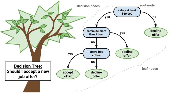
A decision tree is a visual representation that uses branches to demonstrate all possible outcomes of a given decision based on certain conditions. The internal node in a decision tree represents a test on the attribute, each branch of the tree represents the outcome of the test, and the leaf node represents a given class label, i.e. the final decision after computing all of the attributes. The classification rules are represented by a path from the root to the leaf node.

Types of decision trees

i. Classification trees

Used to separate a dataset into different classes based on the response variable. It’s used when the target variable is categorical in nature.

ii. Regression trees

Used when the response variable is continuous or numerical. The end goal is a prediction on a given data problem.

When should we use decision trees?

i. When the target function has discrete output values.

ii. Problems where instances are represented by attribute-value pairs.

iii. Decision trees are robust to errors and are best suited when training data contains errors.

Advantages of decision trees

1. Decision trees are easy to understand and visualize.
2. The algorithm has built-in feature selection which makes it useful in prediction.
3. It can handle both categorical and numerical variables.
4. It saves on data preparation time as it is not sensitive to missing values and outliers.

Disadvantages of decision trees

1. Decision trees lose their predictive power from not collecting other overlapping features.
2. Don’t fit well for continuous variables resulting in instability.
3. Creating large decision trees that contain several branches is complex and time-consuming and doesn’t generalize well to future data.

Applications of decision trees

i. Decision trees are used in the identification of at-risk patients and disease trends.

ii. By the finance sector to classify loan applicants by their default probabilities.

iii. Remote sensing in pattern recognition.

Python Implementation

# Python code for Decision Tree
from sklearn.tree import DecisionTreeClassifier
model = DecisionTreeClassifer()
model.fit(X,y)
predicted = model.predict(X_new)

Random Forest

A random forest is an ensemble of decision tree classifiers. It uses a bagging approach to create a bunch of decision trees with a random subset of data. A model is then trained on the subset of the dataset to achieve better prediction accuracy.

The output of all the decision trees in the random forest is combined to make a final prediction. The final prediction of a random forest is obtained by averaging or polling the results of each decision tree or selecting the prediction that appears most.

Advantages of random forests

1. It maintains accuracy when there are missing data, and it’s resistant to outliers.
2. It’s open-source—there are free implementations of the algorithm in Python and R.
3. One of the most effective and versatile algorithms for a variety of classification and regression tasks.
4. Random forests tend to have higher classification accuracy.

Disadvantages of random forests

1. When using a large number of decision trees, it becomes difficult to interpret and slows the computation process.
2. When used for regression problems, random trees don’t predict beyond the range of response values in the training data.

Applications

• In the automobile industry, to predict failures or breakdowns of a mechanical part.
• In the health care industry, to predict whether a patient will develop a chronic disease or not.

Python Implementation

# Python code for Random Forest
from sklearn.ensemble import RandomForestClassifier
model = RandomForestClassifier()
model.fit(X, y)
predicted = model.predict(X_new)

Conclusion

We should now be having a better understanding of some of the most commonly-used algorithms for machine learning.

There is no best ML algorithm. It’s most important to understand the data at your disposal by asking it the right questions. The answer to these questions lies in the algorithms we’ve discussed. A good rule of thumb is that good data beats better algorithms.