Backpropagation is one of the primary things one learns when one enters the field of deep learning. However, many people have a shadowy idea of backpropagation as it is explained in many beginner-level courses as an intuitive way of following gradients of the loss function through the layers, but seldom referenced mathematically.
Wherever mathematics is involved (especially in deep learning resources and papers) things get a bit too complex and equations are expected to explain themselves at times. Deep learning nowadays is no longer restricted to students at graduate school or research scholars, but is also explored by undergraduates — who tend to skip the mathematical part as it often seems boring.
I will try to bring forth an easier and broken down approach of explaining backpropagation mathematically. As such, I have written this in a way so that people who have just a basic idea of calculus can understand the complete mathematics behind backpropagation. Many of my ideas here are derived from Efficient Backprop [1] as I spent a great deal of time learning about it.
Let us have an artificial neural network module with n layers. Each layer ‘i’ has a weight of ‘Wi’ and outputs are calculated by matrix multiplications between inputs and weights. So, for instance, if we set up the input to the artificial neural network as ‘X0,’ then we have the output of the first layer as:

Where ‘X0’ is the input to the module, ‘W1’ is the weight for the first layer and ‘F1’ is the activation function for the first layer.
So, the output of the nth and last layer of a network can be defined as:

Where ‘X(n-1)’ is the input to the layer ‘n,’ ‘Wn’ is the weight for the layer ‘n’ and ‘Fn’ is the activation function for the same layer.
Now, let us define a loss function ‘L’ that compares the outputs ‘Xn’ with the ground truth ‘G.’ So, the error ‘E’ can be expressed as:

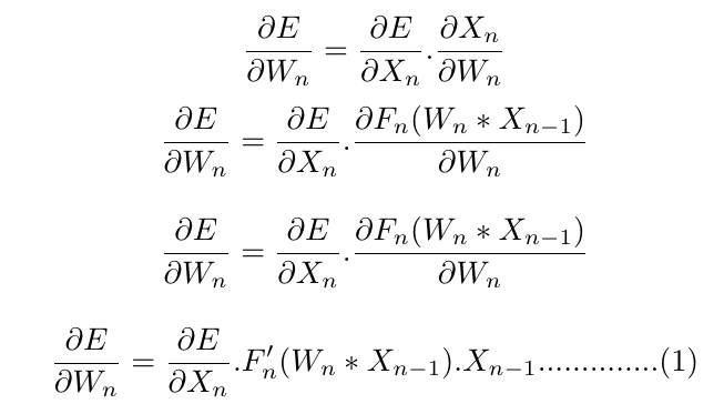
Differentiating with respect to weight ‘Wn,’ we get:

Note that only the weights of the nth layer will be updated on the basis of the derivative of the loss with respect to ‘Xn’ and the previous ‘Wn’ values are used to calculate the equation (1). Essentially, all of ‘Xn,’ ‘Wn,’ and ‘X(n-1)’ are stored prior to weight update of the nth layer and then pushed into this equation to calculate the gradients.
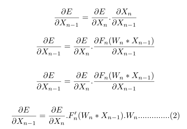
Again we have:

So in this manner, what we do is effectively calculate derivative of loss with respect to ‘X(n-1)’ and bingo — we can now calculate the weight of the (n-1)th layer with the help of something like this equation (1). It is important to note here that ‘Wn’ does not update as soon as the gradient is calculated, it waits for the gradients of all of the weights to be calculated and then all the weights are updated together. As a result of this, the ‘Wn’ term in the equation (2) still points to the weights before the update.
Summary
Backprop itself is dynamic, with the gradients being updated at every call. However, to simplify things, think of it as this static process per call where we effectively store:
- All of the inputs and outputs of the various layers ‘Xn,’ ‘X(n-1),’ ‘X(n-2),’ and so on.
- All of the calculated derivatives of the loss with respect to the inputs at different layers.
- All of the weight values before an update.
Once everything is stored and calculated, depending on the learning rate () and the regularization term, all the weights are updated at once as:

After this, the forward pass is again made — the updated weights are used — and their gradients are then computed again. This loop goes on and on.
Now let’s get our hands dirty with code — let’s implement backward from scratch for a linear layer on NumPy.
Implementation
Let’s look at the implementation of forward and backward passes of a linear layer. The linear layer is a simple layer that has a matrix weight and a bias. Let’s look at their shapes to get a better idea of how they stand:

So the weight is a 512×1024 matrix while the bias is a 512 size vector. But wait — the weight matrix expects the input to have a shape of (N,512), but our input should be a tensor of shape (N,1024) — as in_features=1024 ! This is where the transpose comes in. What we multiply with the input is nothing but a transpose of the weight matrix. Why? Well it varies from framework to framework and this particular framework works out things like this.
Dubbing the transpose of weight of this layer as W0 and the bias as b0, we have X1=(W0*X0)+b0. Let’s implement the forward and backward passes of a linear layer using NumPy now:
    import torch.nn
    import torch

    class Module():
        def __call__(self, *args):
            self.args = args
            self.out = self.forward(*args)
            return self.out

        def forward(self): raise Exception('Not Implemented Error')
        def backward(self): self.back(self.out, *self.args)

    class Lin(Module):

        def __init__(self,w,b):

            self.bias=b
            self.weight=w

        def __call__(self, inp):
            self.inp = inp
            self.out = [email protected] + self.bias
            return self.out

        def back(self,out,inp):
            inp.g= out.g @ self.weight.t()
            self.weight.g = (inp.unsqueeze(-1) * out.g.unsqueeze(1)).sum(0)
            self.bias.g = out.g.sum(0)

    if __name__=='__main__':

        ##Init##
        in_features=1024
        out_features=512
        w1 = torch.randn(in_features,out_features)/math.sqrt(m)
        b1=torch.zeros(out_features)
        ##Init##

        linear=Lin(w1,b1)
        print(linear.weight.shape,linear.bias.shape)
As you can see, we have implemented in the backward pass the exact mathematical form of the gradient discussed in the section above. And does this work? Absolutely! Try pairing it with a simple loss function and build your entire neural network code — completely from scratch! In case you need help with implementation, reach out.
In order to get faster updates, subscribe to my blog 😉
Hmrishav Bandyopadhyay is a 2nd year Undergraduate at the Electronics and Telecommunication department of Jadavpur University, India. His interests lie in Deep Learning, Computer Vision, and Image Processing. He can be reached at — [email protected] || https://hmrishavbandy.github.io

Comments 0 Responses