Positive and Unlabelled Learning: Recovering Labels for Data Using Machine Learning

Problem

It’s often the case that companies want to implement machine learning for a given task—let’s say, to perform classification on data—but are cursed with the problem of having insufficient or unreliable labels for that data.

In these cases, companies could opt to hand label their data, but hand labelling can be a demanding task that could also lead to human bias or significant errors. What if it’s the case that you have labelled data for your positive class, but you have unreliable labels for your negative class? How do you get around this problem?

Positive and Unlabelled Learning.

Heres an example situation:

1000 total samples
100 of them are samples you can consider as reliably positive
900 of them could be unreliable negatives or unlabelled samples
There could be some positives lingering in these

Solution

PU learning, which stands for positive and unlabelled learning, is a semi-supervised binary classification method that recovers labels from unknown cases in the data. It does this by learning from the positive cases in the data and applying what it has learned to relabel the unknown cases.

This approach provides benefits to any machine learning problem that requires binary classification on unreliable data, regardless of the domain.

There are two main approaches to applying PU learning. These include:

PU bagging
Two-step approach

PU Bagging Explained

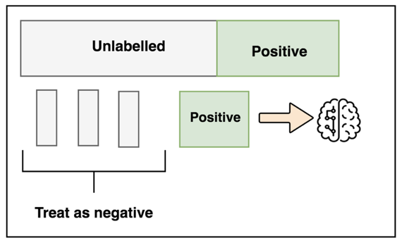
PU bagging is a parallelized approach that takes random subsamples of the unknown cases and creates an ensemble of weak classifiers to output a score for each sample. The steps include:

Randomly sampling subsets of the unknown data and all positives to create an evenly-balanced training set.
Building an ensemble of classifiers with this “bootstrapped” dataset — treating positive as 1 and unknown as 0
Predicting probability scores of unknowns that were not sampled in training — known as the out-of-bag samples (OOB)
Repeat many times and calculate the average OOB scores

Two-Step Approach Explained

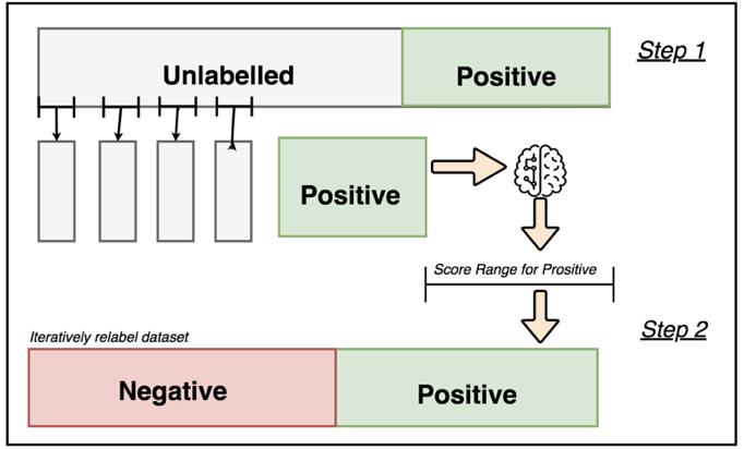
The two-step approach is a more complex method for PU learning that uses machine learning techniques to relabel data while training. The steps for implementation are as follows:

Step one

Train a standard classifier on positive and unknown cases.
Get a score range for definite positive cases to label definite negatives

Step Two

Train a second classifier on your newly labelled dataset and repeat this process iteratively until an established criterion is met.

PU Learning in Action

In order to showcase this, I will work through a small example using the Banknote dataset. It’s a dataset that has 2 classes: unauthentic and authentic, denoted by 0 and 1, respectively.

The background of the dataset isn’t all that important because we aren’t going try to do any feature engineering or classification on a test set. Instead, we’re going to simulate a situation in which there are some reliable positive cases and many unreliable negatives (could be a mix of positive and negatives). Okay, lets get to it!💪

To get started, I’ll import the data and inspect it to see the original label value counts and see if there are any null values:

df_raw = pd.read_csv('data_banknote_authentication.txt', 
                     names=['variance', 'skewness', 'kurtosis', 'entropy', 'authentic'])
print(df_raw.authentic.value_counts())
print('Has null values:', df_raw.isnull().values.any())


'''
Output:

0    762
1    610
Name: authentic, dtype: int64
Has null values: False
'''

variance,skewness,kurtosis,entropy,authentic
3.62160,8.6661,-2.8073,-0.44699,	0
4.54590,8.1674,-2.4586,-1.46210,	0
3.86600,-2.6383,1.9242,0.10645,	0
3.45660,9.5228,-4.0112,-3.59440,	0
0.32924,-4.4552,4.5718,-0.98880,	0

Let’s simulate a scenario of unreliable data—first, we’ll balance the data evenly to have 610 of class 0 and 610 of class 1. Then, we’re going to mislabel some of the positive classes as negative (essentially hiding them) to see if the models can recover them.

def random_undersampling(tmp_df, TARGET_LABEL):
    df_majority = tmp_df[tmp_df[TARGET_LABEL] == 0]
    df_minority = tmp_df[tmp_df[TARGET_LABEL] == 1]

    # Downsample majority class
    df_majority_downsampled = resample(df_majority, 
                                       replace=False,              # sample without replacement
                                       n_samples=len(df_minority), # to match minority class
                                       random_state=None)        # reproducible results
    # Combine minority class with downsampled majority class
    df_downsampled = pd.concat([df_majority_downsampled, df_minority])

    print("Undersampling complete!")
    print(df_downsampled[TARGET_LABEL].value_counts())
    return df_downsampled
  
df_downsampled = random_undersampling(df_raw, 'authentic')
df_downsampled = df_downsampled.sample(frac=1) #Shuffle the data
df_downsampled = df_downsampled.reset_index() #Reset the index
df_downsampled = df_downsampled.drop(columns=['index']) # Drop original index col


# Make a new df because we will need that for later
df = df_downsampled.copy()

#Separate cols from label
NON_LBL = [c for c in df.columns if c != 'authentic']
X = df[NON_LBL]
y = df['authentic']

# Save the original labels and indices
y_orig = y.copy()
original_idx = np.where(df_downsampled.authentic == 1)

# Here we are imputing 300 positives as negative
hidden_size = 300
y.loc[
    np.random.choice(
        y[y == 1].index, 
        replace = False, 
        size = hidden_size
    )
] = 0

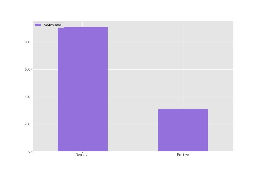
As seen above, 300 out of the 610 true positives were mislabelled as negative. The reason for this is that we want to see if our PU learners can recover them. So to summarize what I did:

1220 samples and 4 features
610 positive out of 1220 before hiding labels
310 positive out of 1220 after hiding labels

To start, let’s set a benchmark. I’m going to train a standard random forest classifier and then compare the result to the original labels to see how many it recovers.

#First random forest
rf = RandomForestClassifier(
    n_estimators = 50,  
    n_jobs = -1           
)
rf.fit(X, y)

print('---- {} ----'.format('Standard Random Forest'))
print(print_cm(sklearn.metrics.confusion_matrix(y_orig, rf.predict(X)), labels=['negative', 'positive']))
print('')
print('Precision: ', precision_score(y_orig, rf.predict(X)))
print('Recall: ', recall_score(y_orig, rf.predict(X)))
print('Accuracy: ', accuracy_score(y_orig, rf.predict(X)))

As you can see, the standard random forest didn’t do very well for predicting the hidden positives. Only 50% recall, meaning it didn’t recover any of the hidden positive classes. Let’s extend this further by jumping into PU bagging.

PU Bagging

If you’ll recall from the explanation above, PU bagging is an approach for training many ensemble classifiers in parallel. In a nutshell: it’s basically an ensemble of ensembles. With each ensemble, the classes are balanced to the size of the positive class. This script written by Roy Wright is a great implementation of PU bagging, so we’ll be using it as a wrapper:

bc = BaggingClassifierPU(RandomForestClassifier(n_estimators=20, random_state=2019), 
                         n_estimators = 50, 
                         n_jobs = -1, 
                         max_samples = sum(y)  # Each training sample will be balanced 
                        )
bc.fit(X, y)

print('---- {} ----'.format('Bagging PU'))
print(print_cm(sklearn.metrics.confusion_matrix(y_orig, bc.predict(X)), labels=['negative', 'positive']))
print('')
print('Precision: ', precision_score(y_orig, bc.predict(X)))
print('Recall: ', recall_score(y_orig, bc.predict(X)))
print('Accuracy: ', accuracy_score(y_orig, bc.predict(X)))

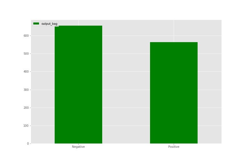
This approach recovered 578 positive samples out of the 610 (95% recall). Pretty good if you ask me 😊 Let’s take a look at this visually:

Imagine implementing this on a huge dataset with millions of rows that are unreliably labelled. Being able to recover them efficiently is a very useful technique to have. Isn’t that cool?👌🏼

Two-Step Approach

For the two-step approach, it’s going to be a little more complicated to implement than for bagging. To put it most simply, what we need to do is:

Identify a subset of of the data that can be confidently labelled as negative (reliable negatives).
Use reliable negatives and reliable positives on a classifier and use that to label unknown samples.

But it’s not always the case that you have reliable negative cases in your dataset. You only have positive and unknowns. To mitigate this you need to:

Train a classifier on positive and unknown cases.
Make a probability range using a predict_proba() function, from lowest-to-highest scores found for positive cases.
Relabel the dataset as positive and negative with all the samples that fall into that score range.
Train a second classifier on the newly labelled data

First, we’re going to create a new target vector with 1 for positive, -1 for unknown, and 0 for “reliable negative” (there are no reliable negatives to start with).

print('Converting unlabaled to -1 and positive to 1...')
ys = 2 * y - 1

# Get the scores from before
pred = rf.predict_proba(X)[:,1]

# Find the range of scores given to positive data points
range_pos = [min(pred * (ys > 0)), max(pred * (ys > 0))]

print('Relabelling unknowns in score range as positive...')
# STEP 1
# If any unlabeled point has a score above all known positives, 
# or below all known positives, label it accordingly
iP_new = ys[(ys < 0) & (pred >= range_pos[1])].index
iN_new = ys[(ys < 0) & (pred <= range_pos[0])].index
ys.loc[iP_new] = 1
ys.loc[iN_new] = 0

Now that we’re done step one, we can move on to step two. For this, we’ll need to initialize a classifier (In this case a standard random forest) and then iteratively retrain the model with the new probability range for the positive class.

tsa = RandomForestClassifier(n_estimators = 50, n_jobs = -1)

for i in range(15):
    print('Iteration: ', i)
    # If step 1 didn't find new labels, we're done
    if len(iP_new) + len(iN_new) == 0 and i > 0:
        break
    
    print('Step 1 labeled %d new positives and %d new negatives.' % (len(iP_new), len(iN_new)))
    print('Doing step 2... ', end = '')
    
    # STEP 2
    # Retrain on new labels and get new scores
    tsa.fit(X, ys)
    pred = tsa.predict_proba(X)[:,-1]
    
    # Find the range of scores given to positive data points
    range_P = [min(pred * (ys > 0)), max(pred * (ys > 0))]
    
    # Repeat step 1
    iP_new = ys[(ys < 0) & (pred >= range_P[1])].index
    iN_new = ys[(ys < 0) & (pred <= range_P[0])].index
    ys.loc[iP_new] = 1
    ys.loc[iN_new] = 0

This is complete when the classifier reached one of two criteria: it can’t find any new labels or when the loop completes. However, I should add that when using this on a big dataset with large parameters (n_estimators) this training can take a long time. Let’s check to see how well it did.

print('---- {} ----'.format('TSA'))
y_hat_val = tsa.predict(X)
y_hat_val = [x if ((x==0) or (x==1)) else 0 for x in y_hat_val] # Convert leftover unknowns as negative

print(print_cm(sklearn.metrics.confusion_matrix(y_orig, y_hat_val), 
labels=['negative', 'positive']))
print('')
print('Precision: ', precision_score(y_orig, y_hat_val))
print('Recall: ',    recall_score(y_orig, y_hat_val))
print('Accuracy: ',  accuracy_score(y_orig, y_hat_val))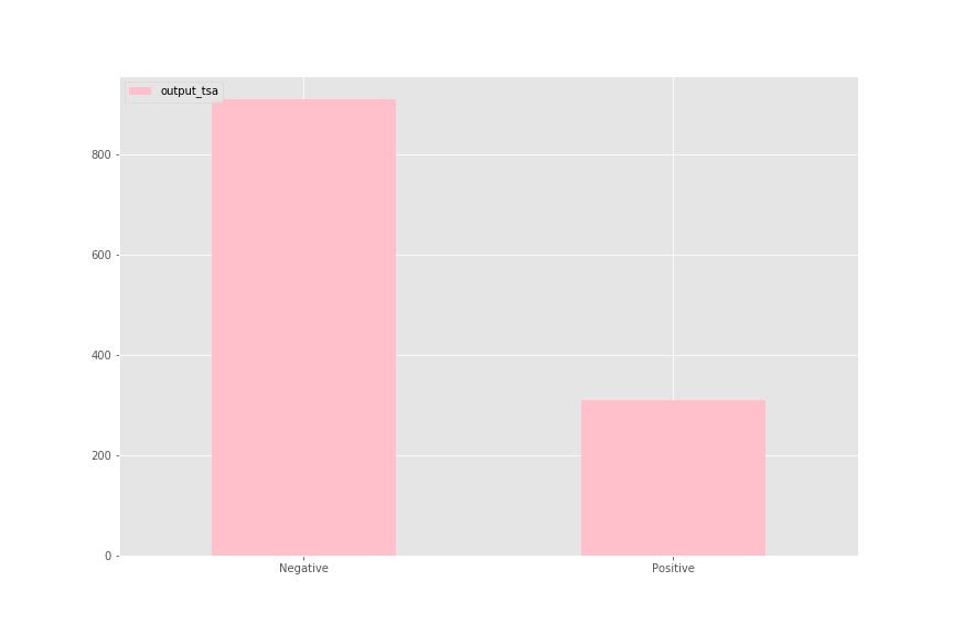

In this case, the TSA model did not perform as well as the PU bagging model. However, with some feature engineering and more data, it may prove that this approach is not as futile as it seems at first glance.

Where is PU Learning Applicable?

These methods can be applied to many areas, one example of which is in detecting spam emails — where you’d want to find positive cases of spam within the unknown samples (IE: spam emails that were not originally caught as spam).
It can also be used as in recommender systems — Let’s say a person uses your website that sells clothes. There is a functionality for liking certain items they’re interested in. It’s possible to use the data of the items a customer likes (true positives) to find new items that they could like (potential positives).
This is just to name a few. There are many other domains in which this method can be used.

Conclusion

Not all datasets are correctly labelled. Even worse, some datasets may not be labelled at all, but with some domain knowledge and through informed weak supervision, a useful machine learning model can still be implemented.

PU bagging is quicker than normal ensemble methods (with tree-based algorithms), as it makes use of parallelization.
TSA takes longer to train.
Remember: this is a pre-processing step, and it’s probably best not to rely on this for your classification problem, in comparison to deep learning methods, which will provide better results.

So what can you do now? If your data consists of unreliable classes, you can use one of these models to predict a probability of a samples’ correct class, and then reassign a new label based on a threshold (ex: if probability > 90% then relabel this row as positive).

Enjoy! 👍

Appendix

I provided all the code on my GitHub. Also, here is a great post, which I took references from.

Code: https://github.com/AaronWard/PU-learning-example
LinkedIn: https://www.linkedin.com/in/aaronjward/
Data Source: http://archive.ics.uci.edu/ml/datasets/banknote+authentication