Recently, there has been a huge rise in the implementation of artificial intelligence solutions, with new deep learning architectures being built and deployed across various industries. This rise could be attributed to two important factors:
- Availability of Computational Power (eg: GPUs, AWS / Digital Ocean Instances)
- Availability of Training Datasets (eg: MNIST, ImageNet, Fashion MNIST)
Deep learning works primarily because of the vast amount of input data on which the deep neural net is trained. Hence, having a good labeled training dataset marks the first step in developing a highly accurate AI solution.
Preparing labeled training datasets for computer vision problems is a painstaking task that involves image processing, manipulation, and finally image labeling. Thus, while dealing with hundreds and thousands of images, programmatic image manipulation and processing stands out as an efficient option for AI dataset creators. So getting familiar with image processing libraries is a convenient first step in creating a custom AI Solution.
ImageMagick
ImageMagick is one such tool, and in fact, it’s one of the most comprehensive open-source image processing libraries. It supports more than 200 image file formats (like: png, jpeg, tiff, pdf) and can display, convert, and edit raster image and vector image files. Jeroen Ooms has been kind enough to develop an R package, magick, that wraps the ImageMagick ST library. Thus, the R-package magick can help R users with advanced image processing.
Installation on Windows and OSX
Since magick is available on CRAN, installing magick is as straightforward as installing any other R-package with install.packages()
Also, the development version of magick is available on ropensci’s GitHub repo and can be installed with install_github() of devtools package.
Please note that for installing from the source (the development version from GitHub), the destination workstation requires RTools.exe to build the source. Also note that the binary CRAN packages work out of the box and have the most important features enabled, which makes installing from CRAN the preferable option.
Installation on Linux
On Linux you need to install the ImageMagick++ library: on Debian/Ubuntu this is called libmagick++-dev:
On Fedora or CentOS/RHEL we need ImageMagick-c++-devel:
Once the installation is successful, the library magick can be loaded into the current R session using library()function.
Reading, Viewing, and Writing Image files
magick supports reading image files from both the local computer or a url on the Internet using theimage_read() function.
Once the image is read into R, it’s basic information, such as image format, dimension, and file size can be extracted using the image_info() function:
If you’re using RStudio (or any other editor with a built-in browser), the read image (inp_img) is automatically displayed in the Viewer after every execution or simply when we mention the image object name (inp_img). In other cases, to view the image, functions like plot() or print() should be wrapped around the magick object to display the image.

Also, the same magick object could be viewed in the default photoviewer application of your system using image_browse()
Similar to image_read() for reading image files into R, image_write() is the function that helps in writing/saving image files in the desired format. The first argument of image_write() is the magick image object into which the image_read() output was saved — in our case inp_img — and the second argument is the path along with the file name where the image has be written/saved. The third argument is the image format in which the image has to be written/saved — like png or svg.
While image_write() can be used for image format conversion — like from .jpeg to .png — magick has image_convert(), which also performs the same image conversion but saves the image object in the memory (the current session) unlike image_write(), which writes/saves the image object to an external file.
As the above output suggests, image_convert() has successfully converted the input jpeg formatted image object into png format but has saved it in memory (in a new R object inp_img_png). And to write the same to an external file, we can use image_write()
Image Enhancements
The core of image manipulation involves performing various image transformations like resizing/scaling the image and applying enhancements, filters, and effects. Most of the time we have to apply enhancements, filters, and effects to the existing raw images in order to improve their appearances or to bring them to desired states.
Of all such enhancements, one primary requirement is the ability to play an image’s color by changing parameters like brightness, contrast, and hue.
image_modulate()
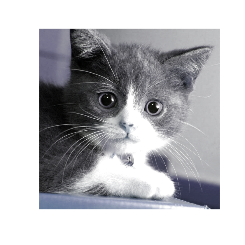
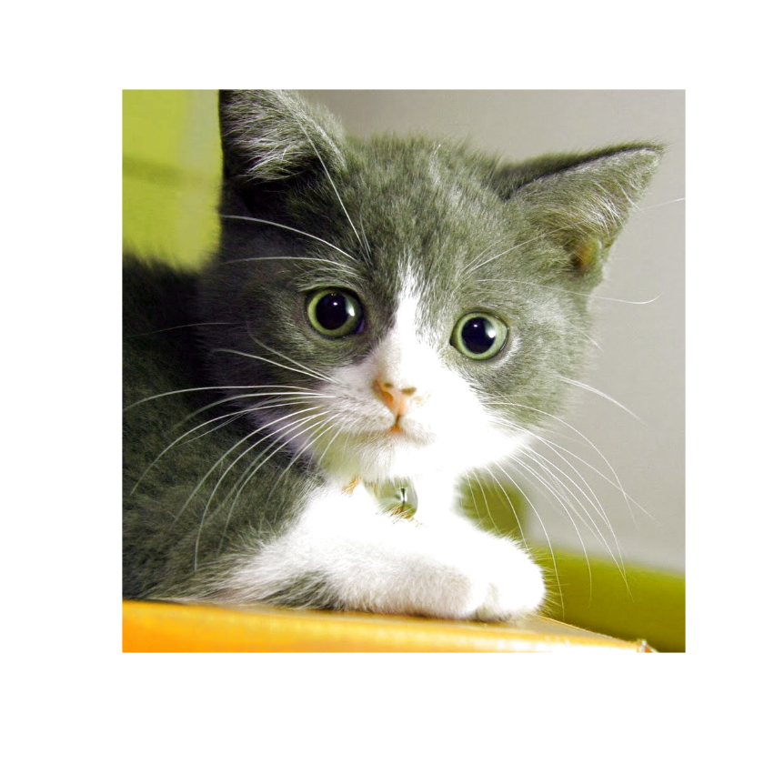
Image Transformation
Let’s begin with the most basic functionalities required in an image editing application: cropping and scaling. magick has two functions with the same name [image_crop() and image_scale()] for cropping and scaling a given image.
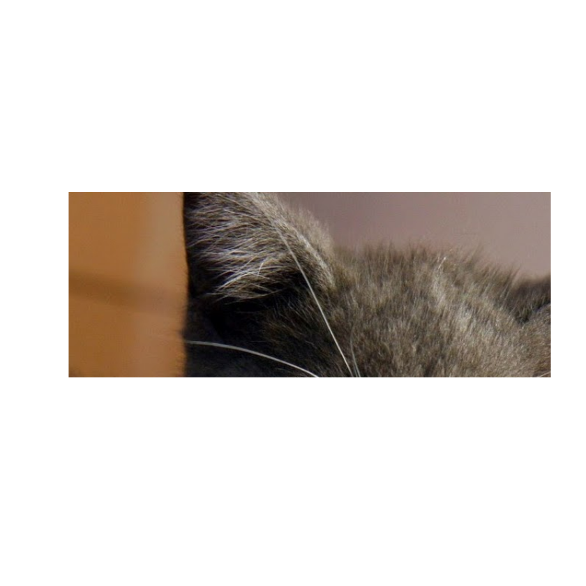
As you can see in the cropped image above, image_crop() crops the input image, taking the given size as its argument. image_scale() acts similarly to image_crop() but scales down/up the entire image to the given size instead of cropping a part of it.

These two functions are very straightforward, but what might look a bit confusing is the way size is passed to these functions. For example, look at this:
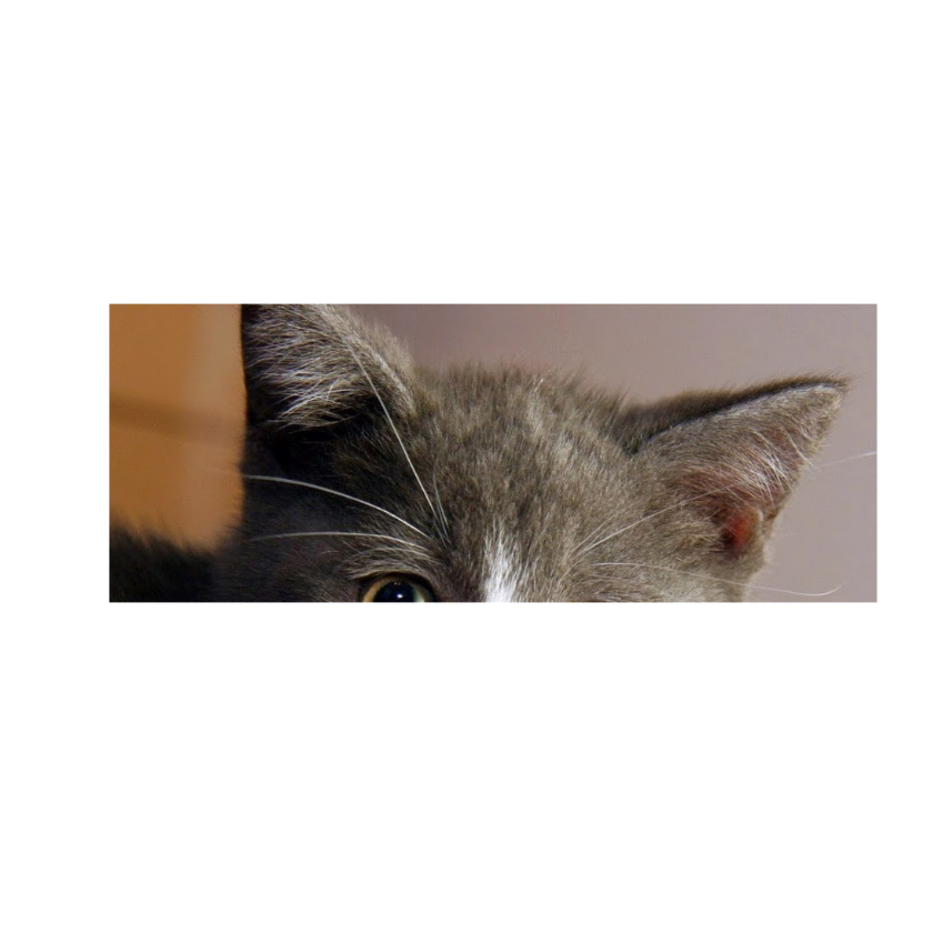
And this:
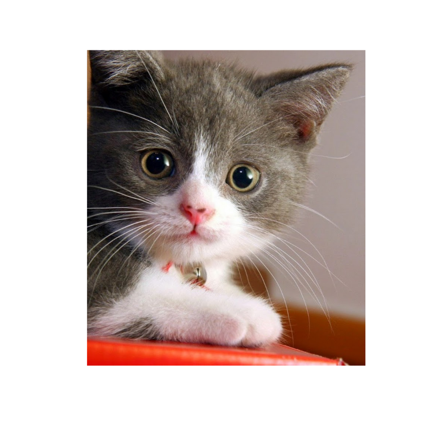
The size value that we pass on these functions is called geometry.
Understanding Geometry
Geometry provides a convenient means to specify a geometry argument. Geometry specification use width, height, xoffset, andyoffset to specify size/dimension and position for an object and is represented in the form of:
Note that, width, height, xoffset, andyoffset are numeric values.
Size — Width and Height
Just like how a dimension is usually represented with x, width and height are used in combination with x to represent the set the size. It’s not mandatory to give both width and height — instead just one of those is sufficient.
For example:
- 200 means width = 200px, so image_scale(image, “200”) will resize the image proportionally to width: 200px
- And without the first number, x200 means height = 200px, so image_scale(image, “x200”) will resize the image proportionally to height: 200px
Offset — x and y
xoffset and yoffset are used with either + or – to offset the image with respect to the left or top edges.
Offset Definition:
- +xoffset : The left edge of the object is to be placed xoffset pixels in from the left edge of the image.
- -xoffset : The left edge of the object is to be placed outside the image, xoffset pixels out from the left edge of the image.
- +yoffset : The top edge of the object is to be yoffset pixels below the top edge of the image.
- -yoffset : The top edge of the object is to be yoffset pixels above the top edge of the image.
Unlike size, both xoffset and yoffset must be provided (i.e., offsets must be given as pairs). The full syntax of geometry is available in the Magick::Geometry documentation.
Now we’ve reached an understanding of basic image transformations like cropping and scaling. But magick has more image transformation functions that follow similar expression styles.
List of Basic image transformations that magick supports:
Applying Filters and Effects
Privacy is a very important factor to consider while collecting data and building artificial intelligent solutions. For example, if Apple or Google is updating their Maps using images captured by their data collection vehicles, it’s important to mask humans or any personal identifying information such license plate numbers. Situations like these are where applying filters and effects plays a vital role. magick has a few standard effects like blur, noise, charcoal and negate.
#blurring level is controlled with two parameters – radius and sigma
image_blur(inp_img,10,5) %>% plot()


Those two functions image_blur() and image_noise() are just two of the many other filters and effects in magick.
List of filters and effects that magick supports:
If you noticed above, all the manipulations we performed on our input image were single-line expressions (i.e., only one operation was performed on the input image).
In a real-life scenarios, we often end up doing a lot more than just one operation, and that’s exactly where the famous pipe operator %>% comes in handy. magick supports the pipe operator %>% to couple multiple expressions (functions, more precisely). If you’re using RStudio, the keyboard shortcut Ctrl+Shift+M types the pipe operator for you.
Let’s look at how to couple more than one image manipulation technique using %>%:
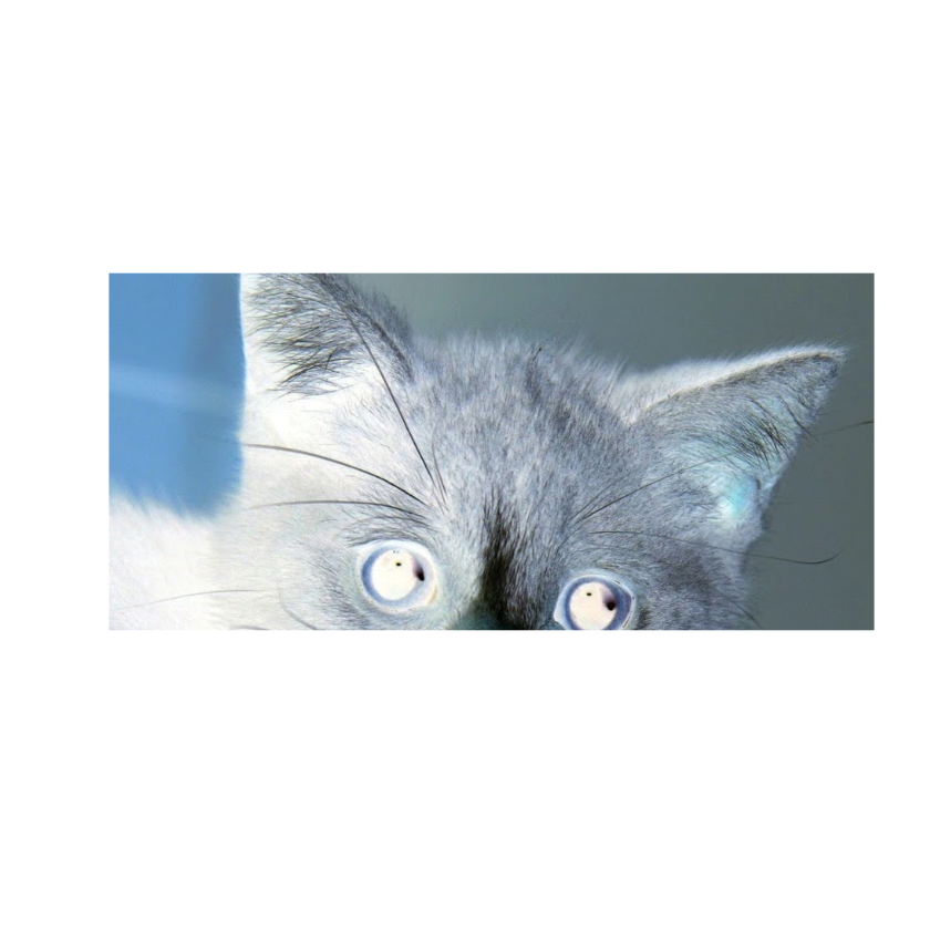
My apologies if the above image looks scary, but the idea is to see how the %>% operator creates a pipeline of functions without the requirement of saving the magick image object after each operation. And of course, the code looks pretty with better readability.
Application of Image Manipulation & Processing in Machine Learning
Computer Vision / AI Dataset Preparation:
For any AI / computer vision problem, the most important component is the input dataset. Creating a new dataset plays a vital role in improving existing state-of-the-art techniques.
The MNIST and ImageNet datasets redefined AI and deep learning, helping researchers develop new neural network architectures and improve accuracy. Thus the application of AI in real-world problems starts with building datasets
In order to use images for building computer vision datasets, images are subjected to a couple of changes, like reshaping all the images into one definite size or converting to grayscale to reduce the number of features (which in turn can reduce training time). That’s where image manipulation and processing techniques that we reviewed above help us.
Below is an example of how a colored image is converted to a grayscale image:
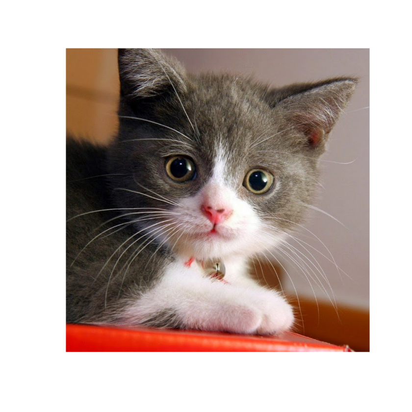
We convert the above color image into a grayscale image using image_quantize(colorspace = ‘gray’)
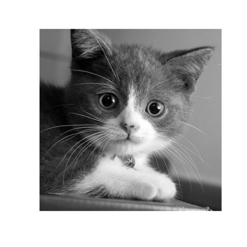
Note that, the process of converting a multicolor image to monochrome (Grayscale) image can also be done using image_convert(type = ‘Grayscale’).
Conclusion
Fei-Fei Li, known for the remarkable ImageNet said,
The purpose of this post is to help you understand how simple image manipulation techniques can come handy in putting together a powerful artificial intelligence / machine learning dataset that in turn can help researchers develop custom AI solutions and better algorithms.
Discuss this post on Hacker News.

Comments 0 Responses