
This article is for anyone that wants to learn the basics of neural networks applied to graphical content, which can be either images or videos.
As an iOS developer myself, I was initially frightened to look into anything related to machine learning. But, one day I stumbled upon a Computer Vision book called Computer Vision – Algorithms and Application by Richard Szeliski. I wouldn’t recommend it for beginners, but it was good introduction for me.
As for any iOS developer, since the release of Core ML and Turi Create, we can definitely build powerful and production-ready ML tools that can enhance the user experience of your application.
In the following post, I’v tried to explain the concept of neural networks the way I would’ve wanted to learn them when I started.
A primer on convolutional neural networks (CNNs)
Nine times out of ten, when you hear about scientific barriers that have been overcome through the application of deep learning techniques, convolutional neural networks are involved. Also called CNNs or ConvNets, they’re the spearheads of deep learning, especially when it comes to computer vision applications.
Today, they’re even able to learn how to sort images by category with, in some cases, better results than manual sorting. If there’s a method that justifies a particular craze when it comes to the deep learning world, then it’s CNNs. What is particularly interesting with CNNs is that they’re also easy to understand, when you divide them into their basic functionality.
A CNN compares images fragment-by-fragment. The fragments a CNN looks for are called features. By finding approximate features that are roughly similar in 2 different images, the CNN is much better at detecting similarities than via a full image-to-image comparison.
These supervised learning techniques can provide very good results, and their performance strongly depends on the quality of the previously-found features. There are several methods for extracting and describing features.
In practice, the classification error is never zero. The results can then be improved by creating new feature extraction methods that are more suited to the studied images, or by using a “better” classifier.
But in 2012, a revolution occurred: at the annual ILSVRC computer vision competition, a new deep learning algorithm surpassed all previous benchmark records! This was a convolutional neural network called AlexNet.
Convolutional neural networks have a methodology similar to traditional methods of supervised learning: they receive input images, detect the features of each of them, and then drag a classifier over them.
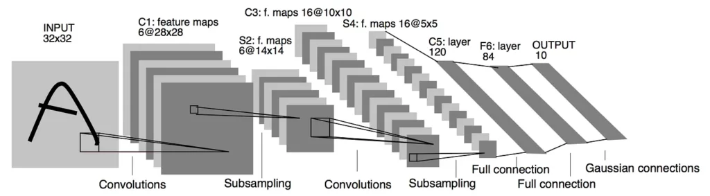
However, features are learned automatically! The CNNs do all the hard work of extraction and description of features: during the training phase, the classification error is minimized in order to optimize the parameters of the classifier AND the features! In addition, the specific architecture of the network can extract features of different complexities, from the simplest to the most sophisticated.
The automatic feature extraction and prioritization, which adapts to the given problem, is one of the strengths of convolutional neural networks: no need to implement a “hand-to-hand” extraction algorithm.
Unlike supervised learning techniques, convolutional neural networks learn the features of each image. That’s where their strength lies: networks do all the work of extracting features automatically, unlike supervised learning techniques.
There are four types of layers for a convolutional neural network: the convolutional layer, the pooling layer, the ReLU correction layer, and the fully-connected layer. Next, I’ll explain the purposes of these different layers.
1. The convolution layer
A convolutional layer is the key component of convolutional neural networks, and generally constitutes at least their first layer.
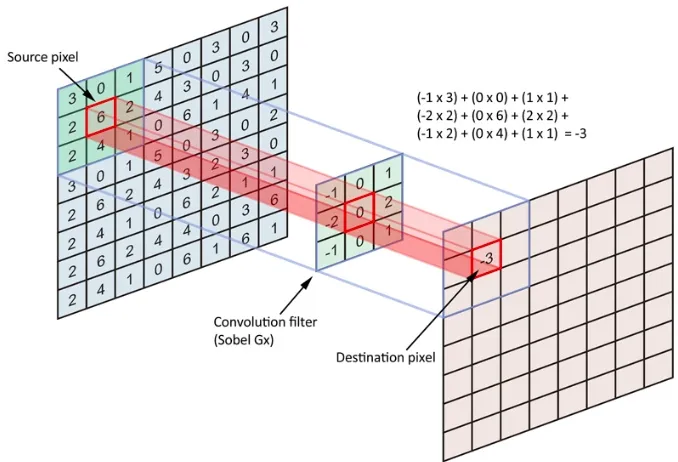
Its purpose is to locate the presence of a set of features in the images received as input. For this, we perform convolutional filtering: the principle idea is to “drag” a window representing the feature on the image and then calculate the product of the convolution between the feature and each portion of the scanned image. A feature is then seen as a filter: the two terms are equivalent in this context.
The convolution layer thus receives several images as input and calculates the convolution of each of them with each filter. The filters correspond exactly to the features you want to find in the images.
We obtain for each pair (image, filter) an activation map, or feature map, which indicates where the features are in the image: the higher the value, the more the corresponding place in the image looks like the feature.
Unlike traditional methods, features are not pre-defined according to a particular formalism (SIFT), but learned by the network during the training phase! The nuclei of the filters denote the weights of the convolution layer. They are initialized and then updated by backpropagation of the gradient.
This is the strength of convolutional neural networks — they’re able to determine all the discriminating elements of an image, by adapting to the problem. For example, if the question is to distinguish cats from dogs, the automatically defined features can describe the shape of the ears or paws.
2. The pooling layer
This type of layer is often placed between two convolution layers: it receives several feature maps as input, and applies to each of them the pooling operation.
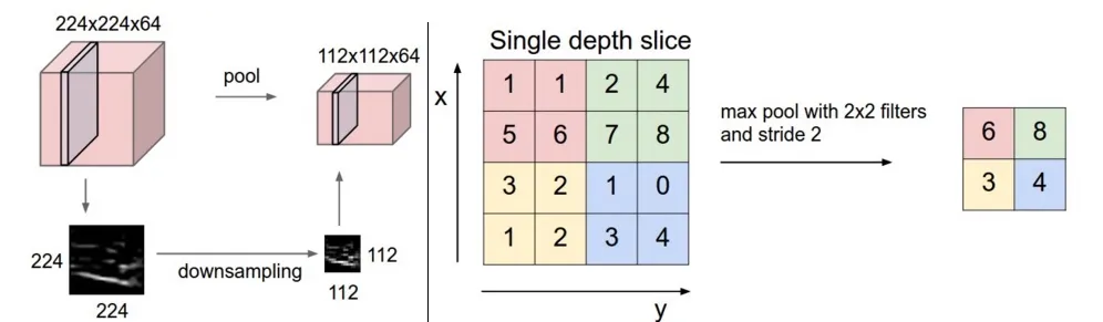
The pooling operation consists of reducing the size of the images while preserving their important characteristics.
For this, the image is cut into regular cells, with the maximum value kept within each cell. In practice, small square cells are often used to avoid losing too much information.
The most common choices are adjacent cells of size 2×2 pixels that don’t overlap, or size 3×3 cell pixels, distant from each other with a pitch of 2 pixels (which overlap).
The same number of feature maps are output as input, but these are much smaller.
The pooling layer reduces the number of parameters and calculations in the network. This improves the efficiency of the network and avoids model overfitting.
The maximum values are spotted less accurately in feature maps obtained after pooling than in those received as input — this is actually a big advantage! Indeed, when you want to recognize a dog for example, his ears don’t need to be located as accurately as possible: knowing that they’re located near the head is enough.
Thus, the pooling layer makes the network less sensitive to the position of features: the fact that a feature is a little higher or lower, or even that it has a slightly different orientation should not cause a radical change in the classification of the image.
3. The ReLU correction layer
ReLU (Rectified Linear Units) denotes the real nonlinear function defined by ReLU(x)=max(0,x).
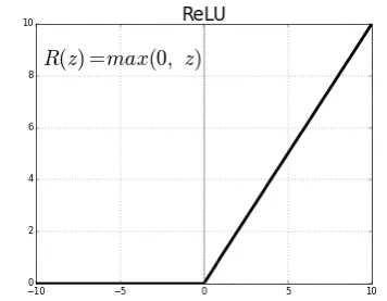
The ReLU correction layer therefore replaces all negative values received as inputs with zeros. It plays the role of an activation function.
4. Fully-connected layer
The fully-connected layer is always the last layer of a neural network, convolutive or not — so it’s not a distinct characteristic of a CNN.
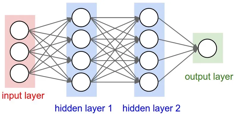
This type of layer receives an input vector and produces a new output vector. For this, it applies a linear combination and optionally an activation function to the values received as the input.
The last fully-connected layer classifies the input image of the network: it returns a vector of size N, where N is the number of classes in our image classification problem. Each element of the vector indicates the probability for the input image to belong to a class.
For example, if the problem consists of distinguishing cats from dogs, the final vector will be of size 2: the first element (respectively, the second) gives the probability of the image belonging to the class “cat” (or, respectively, “dog”). Thus, the vector [0.9 0.1] means that the image has a 90% chance of representing a cat.
Each value of the input array “votes” in favor of a class. The votes do not all have the same importance: the layer gives them weights that depend on the element of the table and the class.
To calculate the probabilities, the fully-connected layer therefore multiplies each input element by a weight, sums it, then applies an activation function (logistic if N = 2 , softmax if N> 2).
This treatment amounts to multiplying the input vector by the matrix containing the weights. The fact that each input value is connected with all the output values explains the fully-connected term.
The convolutional neural network learns the values of the weights in the same way that it learns the filters of the convolution layer: during the training phase, by backpropagation of the gradient.
The fully-connected layer determines the link between the position of features in the image and a class. Indeed, since the input array is the result of the previous layer, it corresponds to an activation card for a given feature: the high values indicate the location (more or less precise according to the pooling) of this feature in the image. If the location of a feature at a certain point in the image is characteristic of a certain class, then the corresponding value in the table is given a significant weight.
Concluding Thoughts
Mobile developers shouldn’t be afraid of ML anymore. With the help of a handful of easy to use libraries, whether in Python or even Swift (Create ML, for example), you can achieve pretty decent results with very little effort.

Comments 0 Responses